Getting Into Reservoir Modeling for Carbon Sequestration

Carbon capture and storage has seen a resurgence, with more companies investing in larger-scale projects. Simulations are required throughout the whole operation from screening of many potential sites to studying specific sites to optimize injection operations and demonstrate regulatory compliance.

This article introduces MRST-co2lab, a free and open-source module in the MATLAB Reservoir Simulation Toolbox (MRST), which can be used to carry out reservoir simulations covering the whole life cycle of a CO₂ project.

We have developed an introductory application that demonstrates basic functionality from the module and can be downloaded from MathWorks' website. This article will go through the application, which progresses from simple calculation of trapping capacities and migration pathways to more detailed reservoir simulations, including complex physical effects.

To run this tool, you need a MATLAB licence and a copy of MRST, which you can download for free from www.mrst.no. An important advantage of a scripted language like MATLAB is that breakpoints can be set, variables can be inspected, and code can be run (and modified) on the fly, which leads to fast implementation and easy debugging. The MATLAB debugger is a great tool in this respect and is immensely helpful when developing MRST code.

Basics of CO2 Trapping

Geological carbon storage involves injection of CO₂ into permeable formations underground. MRST-co2lab is primarily designed to study injection into pristine saline aquifers but storage in depleted reservoirs is also possible. It includes access to publicly available datasets from the CO₂Storage Atlas produced by the Norwegian Petroleum Directorate (NPD). Users can thus load models of potential CO₂ storage sites from the Norwegian Continental Shelf and run the analyses described in this article.

Generally, CO₂ is injected underground in supercritical phase which has density like a liquid but viscosity like a gas. This high-density supercritical CO₂ is ideal for maximizing underground storage. To ensure that CO₂ remains in a dense phase, storage sites are chosen deep enough so they have high enough pressure to stop the CO₂ transitioning back to the gas phase. Supercritical CO₂ is denser than gaseous CO₂, but still less dense than the formation brine. Therefore, any injected CO₂ will rise due to buoyancy. To trap the CO₂ underground, several “trapping mechanisms” come into play.

Stratigraphic trapping. It refers to CO₂ becoming trapped under an impermeable (or less permeable) stratigraphic layer. “Structural trapping” denotes trapping next to a structural feature like a sealing fault or an impermeable formation, displaced along a fault, and juxtaposed with the permeable reservoir.

Residual trapping. It is when CO₂ becomes trapped in the pore space. When CO₂ migrates upward, the heavier formation brine flows in behind it and takes its place. In this situation, capillary forces cause snap-off so that some of the CO₂ is left behind as small, immobile droplets inside the pores and thus becomes trapped.

Dissolution or solubility trapping. It occurs when CO₂ dissolves into the formation brine. This is desirable as brine density is proportional to dissolved CO₂ concentration so CO₂-rich brine will sink, reducing the chance of upward migration to the surface.

Mineral trapping. In this type of trapping, CO₂ forms a weak carbonic acid and reacts with the reservoir rock to precipitate new minerals, which represent the most secure form of storage. The mineralization process can either be very rapid or take a relatively long time compared to the other trapping mechanisms. MRST-co2lab does not model mineral trapping.

Trapping Capacity Estimates in MRST

Site screening requires upper bounds on the storage capacity, often called static estimates since they involve no dynamic simulations. To estimate static storage capacities, MRST-co2lab provides the exploreCapacity()user interface which, when run, launches a GUI window like that shown in Fig. 1. The main plot shows the currently selected geological formation from the CO₂ Storage Atlas. Radio buttons on the upper right enable you to select what information to display in the main plot. The sliders below these buttons enable you to adjust parameters relevant to the trapping estimates.

Fig. 1—Interactive viewer window from exploreCapacity() showing caprock topography, structural traps, and migration pathways (for the Utsira formation).

The resulting storage estimates are shown in the bottom right of the GUI, including a breakdown of the amounts of CO₂ trapped by different trapping mechanisms. Importantly, this is the “maximum theoretical trapping capacity” of the formation assuming that all structural and stratigraphic traps are filled with CO₂, the rest of the reservoir is at maximum residual trapping, and the remaining brine is fully saturated with CO₂.

With this user interface you can quickly investigate static capacity estimates based on rock and fluid properties. For instance, reducing residual CO₂ saturation, by moving the corresponding slider, would result in a reduction in estimated residual trapping capacity and therefore a reduction in total estimated trapping capacity.

Migration Analysis (Spill-Point Analysis)

Supercritical CO₂ migrating up through the formation is analogous to water flowing downwards on a terrain. The difference being that instead of moving downslope and pooling at dips in the terrain, the CO₂ will move upwards and pool under high points in the bounding caprock surface. MRST-co2lab uses simple geometric analysis of the caprock topography to identify migration pathways and potential accumulation points of CO₂. It can be used to display structural traps, spill points, catchment areas that drain into specific traps, and spill pathways that connect the various traps. Because these analyses are computationally inexpensive, you can very quickly identify traps and migration patterns even for large models and use this as the basis for more comprehensive simulations.

To run the analysis, we use the interactiveTrapping() command and pass in a top-surface grid (which is discussed in more detail shortly) or the name of a formation from the NPD CO₂ Storage Atlas.

Fig. 2—User interface from interactiveTrapping() showing catchment areas for all traps in the Johansen formation. With a mouse you can select an injection point and immediately see the accessible traps and migration pathways along with trapping volumes (histogram) and the degree of utilization (pie chart).

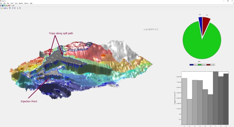
When launched, the viewer displays all traps and their catchment areas. You can now select a plausible well location by clicking in the window. The GUI will then highlight accessible traps and migration pathways along with an estimate of how much structural trapping has been utilized, as in Fig. 2. You can also simulate injection using an efficient vertical equilibrium simulation, which runs much faster than traditional 3D simulations but still gives accurate storage predictions.

Vertical Equilibrium Modeling

Most simulation in MRST-co2lab is carried out using vertical equilibrium (VE) modeling, which assumes instant vertical equilibration of fluids. This is reasonable given the large buoyancy contrast between supercritical CO₂ and brine. VE methods calculate the vertical fluid distribution analytically and only simulate flow numerically in the horizontal directions. Discretizing in two dimensions instead of three reduces run times and memory requirements, making the simulation very efficient.

Setting Up a Simulation Interactively

With the interactive viewer shown in Fig. 3, launched by the command exploreSimulation(), you can interactively set up a simulation to model CO₂ injection and migration and associated pressure build up. Like the interactive trapping viewer, it is possible to load real models from the Norwegian Continental Shelf. Simulation parameters are set by changing settings on the right-hand side of the GUI. Boundary conditions and wells can be placed interactively by selecting the corresponding buttons on the right-hand side and then clicking on the model view on the left.

Fig. 3—User interface from exploreSimulation() showing a VE model of the Utsira formation with 10 injection wells and closed boundary conditions.

VE simulations run in this viewer include advanced effects such as compressibility, a capillary fringe, subscale trapping, and CO₂ dissolution. Trapping inventories showing the amounts of CO₂ trapped via different trapping mechanisms and how these change throughout the simulation are plotted (Fig. 4).

Fig. 4—Evolution of trapping mechanisms over time. Green colors signify CO₂ that will remain trapped unless some process changes the interfacial tension between CO₂ and brine. Yellow color (marginal, in this example) signifies CO₂ that is immobilized inside a trap but could migrate upward if the top seal breaks. Orange and red colors signify mobile CO₂, which either exists inside the migrating plume or has moved out across the model perimeter.

Running a Simulation Via a Script

It is also possible to program a simulation run in a MATLAB script using MRST. To do this, you generally need a grid, data objects for rock and fluid properties, a data object (model) that collects all these structures together and defines the actual equations to be solved, an initial state (pressure and fluid saturations), and a schedule describing the external forces that drive the storage process, i.e., external boundary conditions and well configurations.

To illustrate, we set up a VE simulation of the Johansen formation, offshore Norway. This site will be used for CO₂ storage in the Northern Lights project. Here, we use a simple sector model developed by the NPD and the University of Bergen and later made publicly available by SINTEF under the Open Database License.

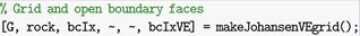
More complete code examples can be found in the online example, but the basic steps are as follows: First, we set up a full volumetric grid containing petrophysical properties using a custom-built function makeJohansenVEGrid(), which also returns a list of the boundary faces where we want to apply a constant pressure boundary condition. There are many ways to make grids in MRST; they can be built from scratch using simple functions such as tensorGrid() or, as here, imported from an industry-standard ECLIPSE input file. There is also functionality for more advanced unstructured gridding and grid refinement; more information can be found here and in the open-access MRST textbook by Lie (2019). The rock structure contains information about porosity and permeability of each cell in the grid.

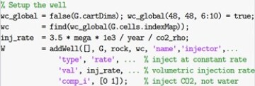
We also need to set up an injection well for the full grid, which we will map to the VE grid later. Here, we want one injection well for CO₂, which we place close to the lowest point in the formation, near the faulted boundary. The well location is given by specifying the indices of grid cells containing the well. In this example we do a nifty trick, and use the IJK topology of the grid to place the well in cells at I, J, K indices 48, 48, and 6:10.

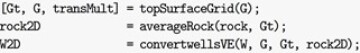
To convert the grid to a 2D VE grid, which represents both the top surface and the underlying rock columns, we use the topSurfaceGrid() function. The averageRock() function calculates the corresponding rock properties by averaging the porosity and permeability values of each column in the grid. Likewise, convertWellsVE() maps well cells from the full grid to the top-surface grid and recalculates the well indices using the new properties. MRST uses a Peaceman type well model, in which well indices control how much flow is induced by the pressure difference between the wellbore and the surrounding grid cell; see chapter 4 of the MRST book for more details on well modeling.

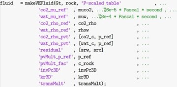
Fluid properties in MRST-co2lab are taken from the CoolProp library. Several choices can be made regarding how the interface between CO₂ and the brine is modeled; details of the different settings can be found in the docstring for the makeVEFluid() function. In our case, we use a capillary-fringe model based on upscaled, sampled capillary pressure. The makeVEFluid() function returns a structure for the fluid, following the standard way of defining fluid properties in MRST.

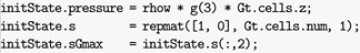
We also need to specify an initial state for the model. In MRST, the state at each timestep is generally a structure containing one field for each primary variable (usually pressure and saturation with fieldnames pressure and s). States returned may also contain other fields such as the intercell fluxes, but to define the initial state it is usually only necessary to specify the primary variables. Here these are pressure, saturation, and the maximum gas saturation a cell has experienced (sGmax), used to calculate residual trapping. We set up the initial state so that the reservoir is initially filled with pure brine and apply a hydrostatic pressure gradient.

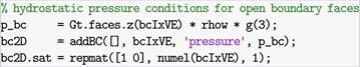
If no boundary conditions are specified on the external faces of the grid, no flow is assumed. It is also possible to set constant pressure or constant flux boundaries. In our example, we set a hydrostatic pressure boundary condition around parts of the edge of the reservoir, identified by the face indices generated by makeJohansenVEGrid().

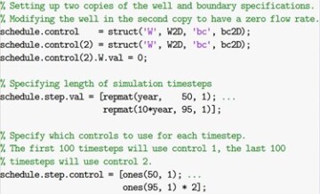
The final thing to create is the schedule. This tells us the timesteps to use for the simulation, which wells are active at which times, and what the boundary conditions are. Our simulation will have two periods, 50 years of injection and then 950 years of post-injection, during which we shut off the well but carry on simulating to see how the system evolves. This is a crucial part of CO₂ storage operations, as regulatory compliance is required well beyond the injection period of a site, and we need to ensure the CO₂ has a low possibility of migration into unexpected areas.

Now we have everything we need to define the mathematical model and run the simulation. The most common approach is to assume isothermal conditions and use a so-called black-oil model from the oil and gas industry, which interpolates viscosities and PVT properties as functions of pressure. We use CO2VEBlackOilTypeModel(), which is a class containing the equations required to run the VE simulation as if it was a normal black-oil simulation, i.e., without worrying too much if it pertains to a VE or a fully 3D model. This is the beauty of the VE formulation, that the VE equations are indistinguishable from the standard black-oil equations and the only things that change are the parameters (e.g., porosity, relative permeability, and capillary pressure).

Then, we feed the model, the initial state, and the schedule into the simulateScheduleAD() function, which will run the simulation and produce the results.

Once the simulation has been run, the example application contains code that animates the CO₂ plume so we can see how it changes through time (Fig. 5).

Fig. 5—Animation showing the plume migration over 1000 years.

We can also calculate the trapping inventories through time to determine which trapping mechanisms are active and how they change throughout the simulation period (Fig. 4).

Summary

Simulation at all stages is critical for the success of CO₂ storage projects. We have presented tools that can be used to easily set up advanced simulation workflows and help simplify decision-making processes. The tools do not offer the full modeling complexity one may need for a real-life business decision but come a long way in an educational or early-stage engineering setting. The rapid simulations enabled by VE-modeling also facilitate studies involving large ensembles, e.g., for assessing parameter sensitivities or scenario optimization. All code is open source meaning it is flexible and cost-effective. In addition, the wide user base of MRST and MATLAB means that these tools are well supported and likely to become more commonplace in the future.