The industry spends significant amount of time and money to optimize completion designs to develop various unconventional resource plays, including cluster spacing or fracture spacing. It is strongly believed that better reservoir characterization and better modeling technique selection ought to shorten the learning curve and save money. This article reviews the state-of-the-art on fracture spacing optimization and discusses the challenges that the industry is facing to achieve an optimal cluster spacing decision.
Introduction
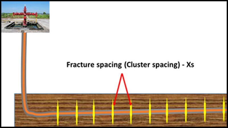
The current technology to develop unconventional resource plays is a horizontal well with multistage hydraulic fracturing treatments. Since permeability is extremely low (<0.001 md) in unconventional resource reservoirs, multiple fractures are needed to have economic well rates, as shown in the image on top (Fig. 1).
Currently, the most popular completion technique is plug-and-perf, where each completion stage includes single or multiple perforation clusters and multiple fractures are initiated from perforation clusters. There are also other techniques, such as sliding sleeve and limited entry perforation to control fracture initiation.
Theory
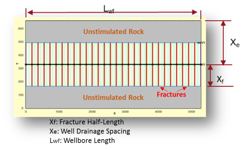
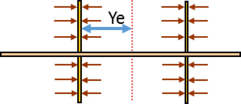
To forecast the well performance, we often set up a planar fracture model like the one shown in Fig. 2. Under the assumption of linear flow with infinite fracture conductivity, Wattenbarger’s Solutions—for “short-term” approximations (Wattenbarger et al. 1998) can be written as the following equation (Eq. 1):
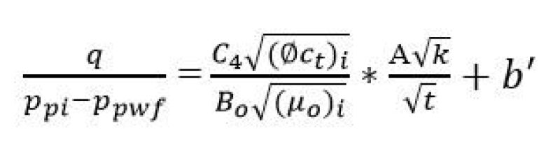
Where “A” is the total fracture surface area, A = 4HfNfXf (Eq. 2)
The Eq. 1 can be simplified as following:
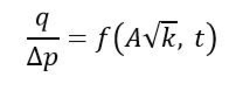
For a given reservoir, the above equation simply states that the well production rate is a function of total fracture surface area and the formation permeability. The total fracture surface area depends on the number of effective fractures. For a given wellbore lateral length, the fracture spacing or cluster spacing decides the number of fracture initiations, and, therefore, decides the well production rate. The above equation explains why the industry is chasing after the fracture spacing or cluster spacing—to increase fracture surface area, thus in order to increase production rate.
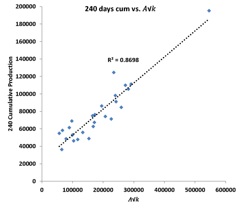
Figure 3 illustrates the analysis results of the\(A{\sqrt{k}}\) vs. 240-day cumulative production from a group of wells located at the Midland Basin, which clearly indicates that the cumulative production is a function of \(A{\sqrt{k}}\), or the fracture surface area and system permeability (permeability within Stimulated Rock Volume (SRV) and initial matrix permeability).
Fluid Flow and Depletion Between Two Fractures
To fully understand the well performance, we study the flow regimes between fractures and horizontal well laterals. The following chart (Fig. 4) illustrates the linear flow regime between two fractures with an assumption of infinitive conductive fractures (meaning no extra pressure drop within fractures).
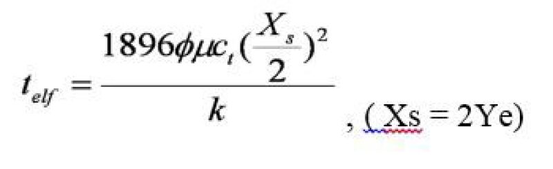
The time to reach the end of the first linear flow can be estimated by the following equation.
To understand the pressure depletion between two fractures, we set up a single porosity model as illustrated in Fig. 4 with initial pressure of 4,500 psi and other parameters as shown in Table 1.
Table 1—Basic model parameters
| Initial Reservoir Pressure (psi) | 4,500 |
| Matrix Porosity | 0.06 |
| Initial Gas Oil Ratio (scf/stb) | 1,000 |
| Oil °API | 40 |
| Hydraulic Fracture Permeability (md) | 10 |
| SRV Permeability (md) | 0.001 |
| Hydraulic Fracture Half-Length (ft) | 200 |
| Constant Flowing Bottomhole Pressure (psi) | 600 |
| SRV Width (ft) | 10 |
Figure 5 illustrates the pressure distributions between two fractures with 40-ft spacing at the end of year 30 for formations with different matrix permeability.
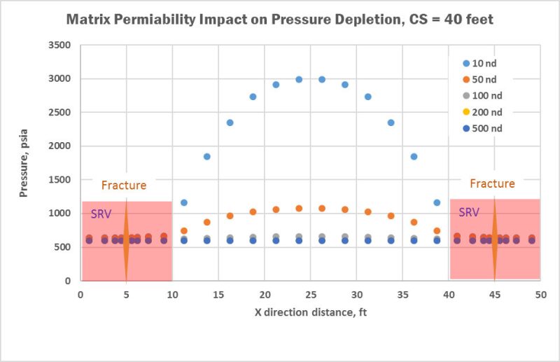
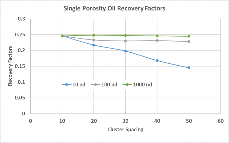
Based upon the modeling results (Fig. 5), one could add more clusters or more fractures if the matrix permeability is around 10 nd. However, for a formation with 100 nd or higher matrix permeability, we can conclude that the 40-ft cluster or fracture spacing is probably too close. We can run a series of different fracture spacing to investigate the recovery efficiency by the end of year 30 as shown in Fig. 6. Both Fig. 5 and Fig. 6 can give us some insights on the pressure depletion and recovery factor for different fracture spacing, which unsurprisingly suggests that the optimal fracture spacing depends on matrix permeability for a given reservoir fluid.
History of Fracture Spacing
More than a decade ago, due to the lack of understanding of unconventional resource reservoirs and the limits of completion technologies, the cluster spacing was designed up to 700 ft in Barnett and Bakken plays. Currently, the cluster spacing is as close as 15 ft apart in Eagle Ford and DJ Basin, and the operators are testing even closer cluster spacing than 15 ft. The motivation of having tight fracture spacing is to have higher initial production rate, as illustrated by Eq. 1. For example, for a horizontal well with 5,000 ft lateral length, we can create 10 fractures with 500 ft fracture spacing, or 100 fractures with 50 ft with the assumption of planar fracture propagation, resulting in 10 times more fracture surface area. With Eq. 1, the initial production rate can be 10 times different provided that all fractures are created equally with the same dimensions and conductivities. Thus, we want to create as many fractures as possible to achieve the highest possible initial production rate. However, higher initial rate is at the expense of possible higher completion cost and operation implementation complexity.
Optimization of Fracture Spacing
Since fracture spacing is so critical, the industry has spent excessive time and significant resources to optimize the fracture spacing. In theory, we can forecast the well performance by building a proper reservoir model with different fracture spacing, fracture properties, and reservoir properties, and then optimize the fracture spacing by tying that with cost and other economic data, provided we have enough data and properly understand the mechanisms of fracturing propagation and fluid flow within nano-darcy rocks. In 2009, Cipolla et.al performed a series of numerical simulations to study the impact of fracture networks on well performance. The study concluded that more complicated fracture network will enhance the well performance. One can interpret the more complicated fracture network as the higher fracture surface area and/or permeability within SRV.
In 2012, Cheng (2012) published a study on the impacts of number of perforation clusters and cluster spacing on production performance. The study focused more on the stress-shadowing effect on the inner fractures, which may have narrower fracture width or less fracture conductivities. Thus, the less conductive fractures would impair the well performance. The study concluded that the magnitude of mechanical interactions of fractures is closely related to the number of fracture simultaneously created and fracture spacing, and that increasing the number of perforation clusters in one stage does not necessarily increase the initial production rate.
Lu et al. (2016) performed a similar study. However, probably due to different assumptions, the study showed the wider middle fractures (higher fracture conductivity) but less fracture dimensions. For the formation case they studied, it was recommended that optimal cluster spacing is about 120 ft. Jin et al. (2013) performed a thorough fracture spacing study with numerical simulations and developed simple correlations that quantify the required fracture spacing necessary to optimize hydrocarbon recovery for different reservoir permeability and fluid properties. The study focused more on the impact of “k/u” (reservoir flow mobility ratio). The study used the fracture or cluster efficiency to simplify the impact of the fracture dimensions and conductivity, and no geomechanical impact was directly included in the study. The study concluded that the fracture spacing would range from 33 ft to 273 ft in Eagle Ford depending on matrix permeability and reservoir fluid properties. The study also recommends increasing the number of stages while reducing the number of clusters per stage, which was derived from the consideration of less efficiency with more perforation clusters within a single completion stage.
All of the studies have concluded that the well performance and economics depend on the number of effective fractures created and connected to the wellbore. The optimal fracture spacing depends on the matrix permeability and the effective drainage surface of hydraulic fractures. The challenges:
Knowing the representative matrix permeability for a given reservoir
Lack of understanding of fracture propagation mechanism and nano-dacy rock fluid flow mechanism
The Challenges and Directions of Efforts
Until recently, we modeled the hydraulic fracturing propagation with the assumption of single planar fracture per cluster (per fracturing initial point). One can easily speculate that the performance of a well with fractures shown in Fig. 7 would be different from a well with multiple planar fractures.
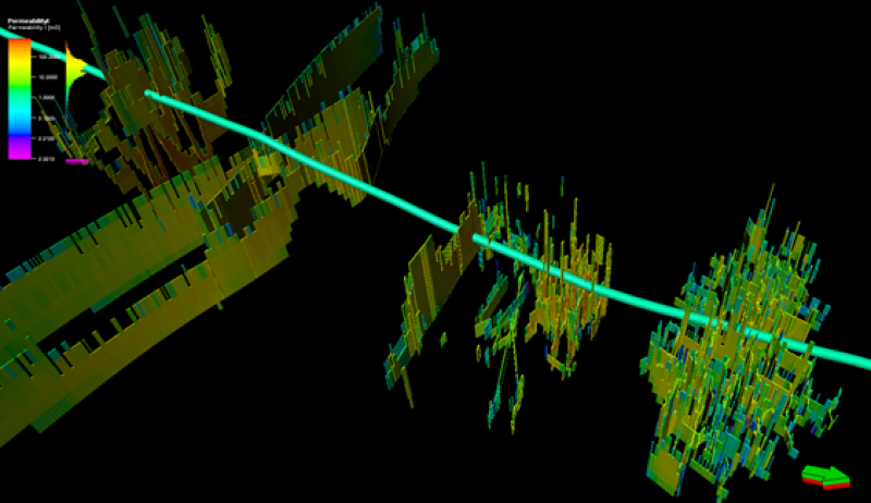
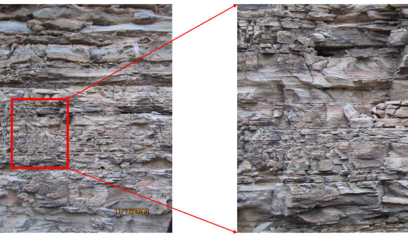
Figure 8 shows a photo from one of Eagle Ford outcrop spots. We can easily see the layering/bedding and heterogeneity. We can speculate that hydraulic fracturing growth is probably much more complicated than planar fractures. Lack of complicated fracture modeling technologies limits our understanding of hydraulic fracture propagations and thus constrains the applications of the “optimal” fracture spacing recommendations from various studies, including those mentioned earlier.
Though a lot of progress has been made to measure the matrix permeability in nano-darcy rock, it has been one of the main bottleneck spot to assess the representative matrix permeability for a given formation. In addition, it is very hard (if not impossible) to estimate the permeability within SRV, which is dictated not only by initial matrix permeability, but also by the rock mechanical properties and completion pumping history.
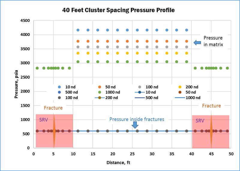
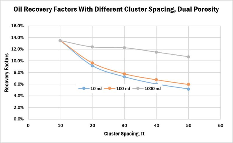
Reservoir characterization plays a significant role in cluster/fracture optimization process. For example, we need to know if a single-porosity model fits a given formation or a dual-porosity model fits the situation better. For the early example shown in Table 1, if we use a dual-porosity model, both pressure depletion (Fig. 9) and recovery efficiency (Fig. 10) are quite different from the ones from a single-porosity model (Fig. 5 and Fig. 6). Based upon the dual-porosity model, the pressure inside fractures is the same as the flowing bottomhole pressure while the pressure in matrix is hardly depleted (Fig. 9) at the end of year 30. The modeling results also tell us that we may want to place the cluster as close as 10 ft, even with higher matrix permeability, which is significantly different from the conclusion based upon the single-porosity model. Therefore, the deep understanding of reservoir characterization dictates the selection of different modeling approaches, which, in turn, will dramatically impact on the selection of the fracture spacing.
Though there have been studies performed to understand the might-be non-darcy flowing mechanisms within nano-darcy rocks (Swami et al. 2013, Yan et al. 2013), most of commercial simulation tools are still based upon Darcy-flow mechanism only. We do not know the impact of using Darcy-flow simulator to model possible non-darcy flows within nano-darcy rocks, which, in turn, limits the application of our current modeling study recommendations. Because of the limitations of fracture spacing recommended by different simulation modeling studies, the industry has spent tremendous resources to pilot-test and optimize fracture spacing and completion size. It may take hundreds of million dollars and long time for an operator to settle down with the “optimal” cluster spacing and completion size whenever it enters a new play. The money and time can be and should be significantly reduced by better understanding reservoirs and better modeling techniques.
Therefore, the industry has been working on different technology fronts so that we can quickly reach an optimal fracture spacing decision for a given formation:
- Matrix permeability: Unsteady-state methods have been developed to measure the matrix permeability in the labs (Jin et al. 2015), and digital rock and other technologies should speed our understanding process and permeability acquisition (Walls et al. 2012, and Rassenfoss 2011)
- In addition to the conventional well logging, the industry is acquiring geomechanical data while drilling, with a module special for rock mechanical properties as a part of drilling bit assembly (Rassenfoss 2016)
- Complicated fracturing modeling technologies are being developed to simulate multistage and multi-cluster fracturing propagation (Cohen et al. 2017, and Izadi et al. 2017)
- To increase the cluster efficiency, new techniques are being employed, including single cluster per stage (Ingle et al. 2017) and extreme limited entry perforation (Somanchi et al. 2017)
- To assess cluster/fracture spacing, fiber-optic cables (such as DAS and DTS) have been deployed along wellbore laterals (Wheaton et al. 2016, Somanchi et al. 2017).
Conclusions
The pressure depletion behavior and recovery efficiency between two fractures depend on the SRV permeability, spacing, and rock mechanic properties, and pre-existing natural fracture network. In addition, selecting proper modeling techniques is crucial to help us get insight into pressure depletion and recovery efficiency.
Effective fracture spacing is critical to well performance. The key to an optimal fracture/cluster spacing decision is reservoir characterization, such as understanding of reservoir matrix permeability, geomechanical properties, and existing natural fracture networks. Great efforts should be taken to understand the reservoir and develop better modeling technologies to reduce the piloting cost and shorten the piloting period to get into full-field development stage. The industry is working in different technology fronts to attack the challenges.

References
SPE 138843 Impacts of the Number of Perforation Clusters and Cluster Spacing on Production Performance of Horizontal Shale-Gas Wells by Y. Cheng.
SPE 124843 Evaluating Stimulation Effectiveness in Unconventional Gas Reservoirs by C.L. Cipolla, E.P. Lolon, and B. Dzubin.
SPE 184876 Stacked Height Model To Improve Fracture Height Growth Prediction, and Simulate Interactions with Multi-Layer DFNs and Ledges at Weak Zone Interfaces by C. Cohen, O. Kresse, and X. Weng.
SPE 185064 Practical Completion Design Optimization in the Powder River Basin by T. Ingle, C. Ketter, D.M. Anderson et al.
SPE 184854 Fully Coupled 3D Hydraulic Fracture Growth in the Presence of Weak Horizontal Interfaces by G. Izadi, D. Moos, L. Cruz et al.
SPE 168813 A Production Optimization Approach to Completion and Fracture Spacing Optimization for Unconventional Shale Oil Exploitation by C.J. Jin, L. Sierra, and M. Mayerhofer.
SPE 175105 Permeability Measurement of Organic-Rich Shale—Comparison of Various-State Methods by G. Jin, H.G. Perez, A.A. Al Dhamen et al.
SPE 184483 Unconventional Reservoir Perforating Cluster Spacing Optimization Method for Staged-Fracturing Horizontal Well by Q. Lu.
S. Rassenfoss 2011. Digital Rocks Out to Become a Core Technology, JPT, May, pp 36–41
S. Rassenfoss 2016. Unconventional Measures for Shale Reservoirs, JPT, May, pp 30–31.
SPE 184834 Extreme Limited Entry Design Improves Distribution Efficiency in Plug-n-Perf Completion: Insights From Fiber-Optic Diagnostics by K. Somanchi, J. Brewer, and A. Reynolds.
SPE 164840 A Numerical Model for Multi-Mechanism Flow in Shale Gas Reservoirs With Application to Laboratory Scale Testing by V. Swami, A. Settari, and F. Javadpour.
SPE 152752 Shale Reservoir Properties from Digital Rock Physics by J. Walls, E. Diaz, and T. Cavanaugh.
SPE 39931 Production Analysis of Linear Flow Into Fractured Tight Gas Wells by R. Wattenbarger, A. H. El-Banbi, M.E. Villegas et al.
SPE 179149 A Case Study of Completion Effectiveness in the Eagle Ford Shale Using DAS/DTS Observations and Hydraulic Fracture Modeling by B. Wheaton, K. Haustveit, W. Deeg, et al.
SPE 163651 Beyond Dual Porosity Modeling for the Stimulation of Complex Flow Mechanisms in Shale Reservoirs by B. Yan, Y. Wang, and J.E. Killough.