Reservoir simulation presents one of the most intimidating challenges a petroleum engineering student encounters, owing primarily to the mathematical complexities involved. The thrust of this article is to capture the basic elements of the simulation process.
In the effort of stay within a logical length, the omission of some details and minor intermediate steps was unavoidable.
Reservoir Model, Simulation Inputs, and Outputs
The main function of a reservoir simulator is to model fluid flow through porous, permeable media, located deep in the subsurface. The spatial domain over which the simulation is performed is divided into a number of interconnected “gridblocks” of geometric dimensions ∆x, ∆y, and ∆z in a classic Cartesian coordinate system (the more the gridblocks, the slower the simulator’s speed, but higher the accuracy).
The simplest modeling approach is the finite differences method (FDM), which ultimately converts a highly-complex partial differential equation (PDE) into a system of linear algebraic equations; one for each node (1 ≤ i ≤ N), connecting it to its surrounding nodes. These algebraic equations are combined together into one matrix-vector expression and are solved simultaneously in each time-step. During every simulation time-step, various reservoir properties (Table 1) are assigned for each node; some inputs staying constant throughout the entire simulation, while others vary following a prescribed model or correlation, such as the Corey and Brooks (1964) and van Genuchten (1980) models for relative permeability and capillary pressure, respectively.

For two-phase, immiscible flow considerations, some reservoir property values (k, kr, μ, B and q) are different for each phase, hence the subscripts, “w” and “o” are used to indicate the respective water-phase and oil-phase values (i.e., kw, ko, krw, kro, μw, μo, Bw, Bo, qw, and qo). Subsequently, processed parameters that are calculated using these properties throughout the simulation will also vary for each phase.
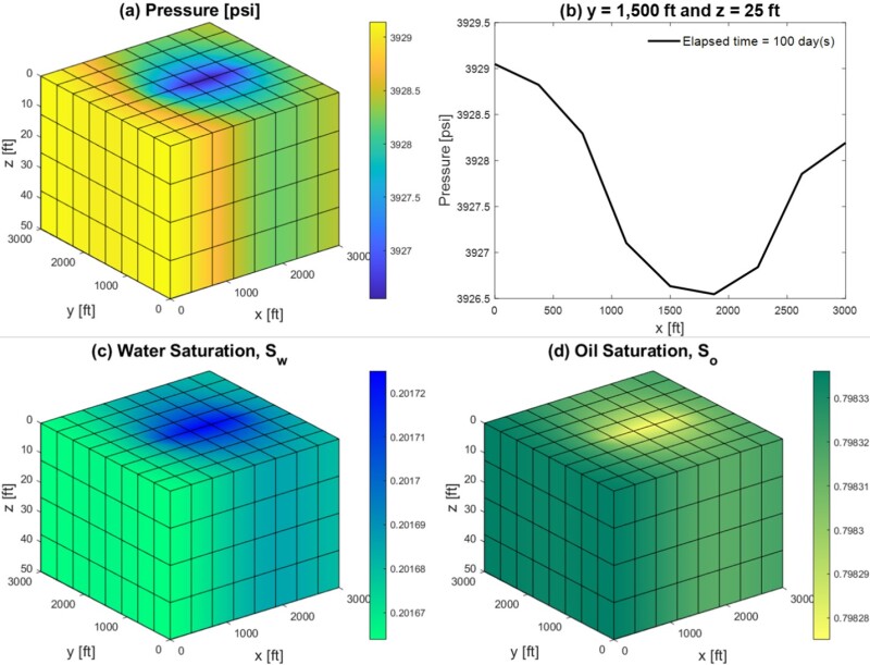
The outputs after every simulation time-step (of duration, ∆t) are in the form of pressure, p, water and oil saturation (Sw and So, respectively) within the predefined spatial domain (Fig. 1), whose values at each node are stored in corresponding output vectors (p, Sw, and So) that get updated following every time-step. The initial conditions (ICs) of these three output vectors must be input a-priori to the first simulation time-step.
Simulation Execution and Stability
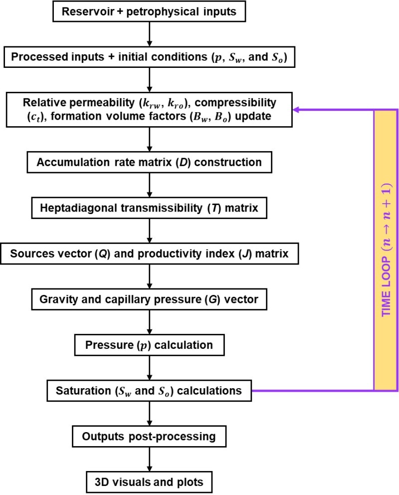
The simplest reservoir simulator execution scheme is IMPES (IMplicit Pressure, Explicit Saturation), which reduces computational effort and facilitates implementation, as it leads to smaller systems-of-equations; one for every node (1 ≤ i ≤ N). Table 2 displays the matrices and vectors involved under an IMPES scheme, besides the output pressure and saturation vectors.

Within the time-loop (Fig. 2) the p vector—containing the pressure value at each node—is first evaluated for the new time-step, n+1 , using its own values from the previous time-step, n:

Next, the Sw vector is evaluated also for time-step, n+1, using the newly-calculated P vector from Eq. (1) by:

Subsequently, using material balance, the So vector is obtained by:

Eqs. (1) and (2) are in the form “Ax=b,” solvable by various numerical methods, such as lower-upper (LU) decomposition. MATLAB’s backslash function is a powerful tool for efficiently solving such systems (i.e. via typing “x=A\b”).
Nevertheless, due to the explicit portion of the IMPES scheme, its stability remains subject to a time-step restriction, requiring that the Courant-Friedrichs-Lewy (CFL) criterion is satisfied for the given conditions (Coats, 2003). The simulator can easily be adjusted for the maximum possible ∆t to be used at all times.
Boundary Conditions and 3D Visualization
Besides ICs, the simulation is subject to boundary conditions (BCs). The most common BCs are (i) constant flowrate “Neumann” and (ii) constant pressure “Dirichlet.” To visualize the behavior of a vertical well producing from a square reservoir subjected to one constant pressure (Dirichlet) boundary, a closed rectangular reservoir, bounded by no-flow (Neumann) boundaries is considered (Fig. 3), de facto simulating two identical square reservoirs joined together. A well produces from the center of the left reservoir at a constant flowrate and another well injects at the same flowrate from the center of the right reservoir, thereby inducing a constant pressure boundary midway (along x = 2,000 ft).
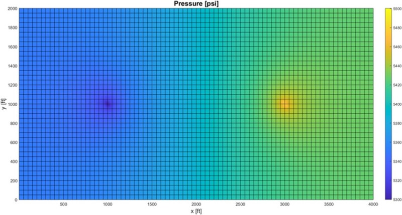
Neumann conditions can be approximated by specifying a flowrate on a reservoir edge. In this vein no-flow conditions can be implemented, mimicking the start of an impermeable zone (e.g., a shale acting as a seal). The best way to approximate a Dirichlet boundary is by creating “imaginary” gridblocks outside of the reservoir edge with specified pressures, so the arithmetic average between an imaginary gridblock and its adjacent (real) gridblock equals to the desired constant pressure.
Incorporating Neumann or Dirichlet BCs requires altering the elements within Q the vector in Eqs. (1) and (2) that correspond to the nodes along the particular boundary. Dirichlet BCs additionally mandate altering the diagonal elements within the T matrix that correspond to the nodes along the boundary.
Tips for Plotting on MATLAB:
Once the simulation is completed, the values from the final output vectors (p, Sw, and So) contain the data necessary for creating visual representations of the reservoir’s state regarding these three properties. MATLAB’s “surf” function can be used to create six 2D surfaces on the edges of the simulated 3D block (Fig. 1). Using the “interp” function, each gridblock’s face can be colored according to the values of its four surrounding nodes.
Verification Exercise
The best way to determine how reliable and accurate a reservoir simulator is, is by performing a simulation with a known solution and comparing the obtained results with that pre-established solution. Once all coding errors and bugs are eliminated, the mesh can be optimized so that acceptable results are produced within a logical simulation speed.
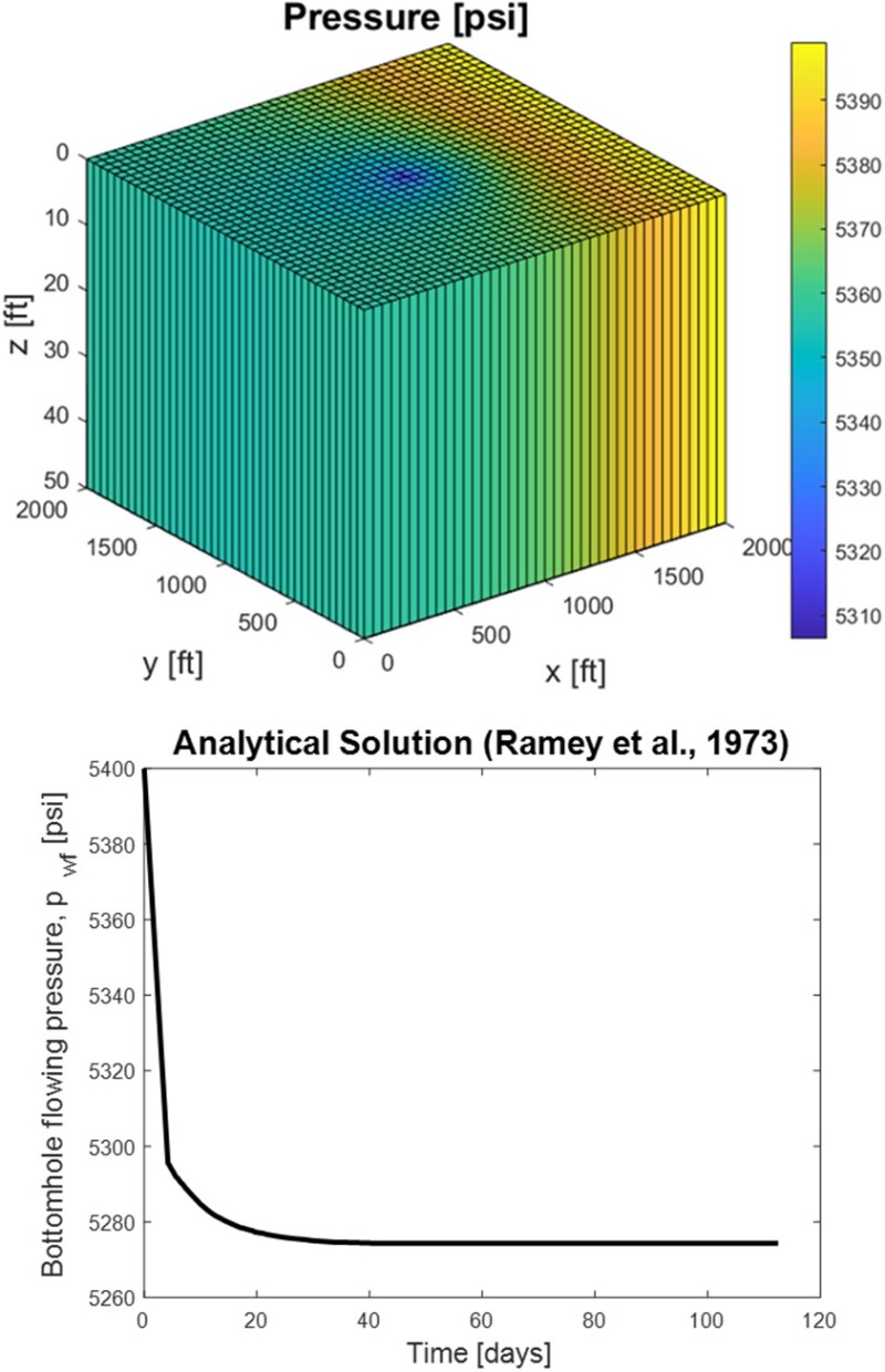
Ramey et al. (1973) derived analytically the solution for the problem of a vertical well of radius, rw = 1 ft, producing water at q = 500 STB/day from the center of a square (2,000 ft × 2,000 ft) reservoir, 50 ft thick, at an initial pressure of 5,400 psi, φ = 0.25, kx = ky = 100 mD, kz = 0, ct = 12×10-6 psi-1, and μ = 1 cp. All boundaries are no-flow, except along x = 2,000 ft, which is kept at constant pressure. Fig. 4 shows the mesh used to numerically model Ramey et al.’s (1973) problem and its analytical solution vis-à-vis the pwf variation with time. For a horizontally isotropic reservoir permeability (kx = ky) and ∆x = ∆y, pwf can be approximated using the pressure at the model’s central node, pcenter following Peaceman (1978) by

The implications of such computational feat are direct. A robust, multipurpose reservoir simulator can easily be adapted to model simple parametric studies, giving immediate numerical results similar to those expensive commercial simulators and can serve as a useful primer for someone’s early exposure to computational reservoir modeling and its peripheral projections.
Acknowledgment
Thanks to Matthew Balhoff, professor, Hildebrand Department of Petroleum and Geosystems Engineering and director, Center for Subsurface Energy and the Environment at University of Texas-Austin for his review of the article.
References
Aziz, K. (1979). Petroleum Reservoir Simulation. Applied Science Publishers, 476.
Balhoff, M. T. (2012). PGE 323M: Reservoir Engineering III (Simulation). Course Notes, The University of Texas at Austin, Aug. 31.
Brooks, R., and Corey, T. (1964). Hydraulic Properties of Porous Media. Hydrology Papers, Colorado State University, 24, 37.
Coats, K. H. (2003). IMPES stability: the CFL limit. SPE Journal, 8 (03), 291–297.
Michael, A. (2021). PIMPS3D2P: A Practical, Efficient, Three-Dimensional, Two-Phase Reservoir Simulator Written in MATLAB. In 82nd EAGE Conference and Exhibition 2021. European Association of Geoscientists & Engineers. Oct 18–21. (Paper accepted for presentation.)
Van Genuchten, M. T. (1980). A Closed‐Form Equation for Predicting the Hydraulic Conductivity of Unsaturated Soils. Soil Science Society of America Journal, 44 (5), 892–898.
Peaceman, D. W. (1978). Interpretation of Well-Bock Pressures in Numerical Reservoir Simulation. SPE Journal, 18 (03), 183–194.
Ramey, H. J., Kumar, A., and Gulati, M. S. (1973). Gas Well Test Analysis Under Water-Drive Conditions. American Gas Association.
Recommended Watching
Video Lectures: A Review of MATLAB and MATLAB Programming