
Artificial intelligence (AI) is a rapidly growing field that is, like electricity, impacting all areas of life, and the petroleum industry is not exempt. Professor Andrew Ng described it as, “AI is the new electricity.”
The research on the application of AI in the petroleum sector has yielded promising results. However, as a petroleum professional, you may be wondering how to implement AI . This four-part series will address that question with a real case study.
This first part will discuss the overview of the basics of machine learning, a subset of AI, and how it can be used to make predictions. By the end of this reading, you will have a clear understanding of how machine learning algorithms predict permeability at a given porosity value or similar parameters. Before diving into the content, it is recommended to allocate at least 1 hour for reading, as the article will delve into the mathematics behind machine learning. Additionally, having a pen and paper on hand is suggested for taking notes.
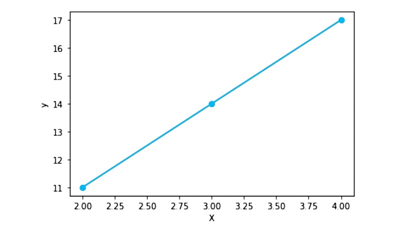
Start with a basic example. Consider a scenario where the input variable (x) is represented by the values: 2, 3, and 4. The output variable (y) is determined by Eq. 1:
y = 3x + 5 (Eq.1)
By plugging each value of x into Eq. 1, we can calculate the corresponding y values: 11, 14, and 17. The relationship between x and y is linear, as illustrated in Fig. 1.
In this example, we assumed that y = 3x + 5. However, in reality, the relationship between the input and output variables is not always known—for example, the correlation between porosity and permeability. All we have is a set of data, as shown in Table 1.

So, how do we determine the relationship between input and output (porosity and permeability) so we can then predict the value of y for future values of x? Machine learning is the answer.
You may recall the equation of a line from high school mathematics: y = mx + c, where m represents the slope and c represents the y-intercept. In machine learning, this equation is rewritten as Eq. 2, where w is the weight, b is the bias term, x is the input, and ŷ is the predicted output, read as y-hat. Remember that y is the real value of the output (given in Table 1) and ŷ is the value predicted by a machine learning model. Also, note that weight and bias (w and b) are called parameters.
ŷ = wx + b (Eq. 2)
The goal of the machine learning model is to find the best values for the parameters weight (w) and bias term (b). From Eq. 1 (y = 3x + 5), we can see that w is 3 and b is 5. Therefore, if our machine learning model finds values of w and b close to 3 and 5, respectively, it will accurately predict the output (ŷ).
First, let’s do it manually to understand the background of how machine learning works. Let's choose w and b randomly. Say both are equal to 1 and try to predict the value of ŷ for x = 2.
ŷ = 1(2) + 1 = 3
From above, ŷ is 3 which is far away from the real value, y = 11, (from Table 1, real value of y at x = 2 is 11). So, w = b = 1 is not a good choice.
Let’s change any one of them or both. If I make both w and b equal to 2. The value of ŷ at x = 2 will be:
ŷ = 2(2) + 2 = 6
Again, not an excellent fit as real value of y is 11.
Similarly, we can try w = b = 2 for other values of x (3 and 4) and you will get a poor match between ŷ (predicted value) and y (real value).
You can come up with as many values as you can for parameters (w and b), both positive and negative, until you get a perfect fit. But this tedious task will take a lot of time and effort to find the best values. However, machine learning can do this for us within a few seconds.
At this point, you understand the job of machine learning (finding the best values of parameters). Let’s dive deep to know how machine learning models find the parameters.
The first step is to select random values for w and b (weight and bias).
Step 1
Let’s initialize the parameters. Say w = b = 0.
Use Eq. 2 (ŷ = wx + b) to find ŷ at given x and w = b = 0.
At x = 2,
ŷ = 0(2) + 0 = 0
At x = 3,
ŷ = 0(3) + 0 = 0
Similarly, at any other value of x, ŷ will be 0, given that w = b = 0.
Step 2
I break down Step 2 into three parts. The first part is to find the difference between the ŷ (predicted values) and y (real values).
At x = 2, ŷ is 0 and y is 11, so the difference (ŷ – y) is -11.
At x = 3, ŷ is 0 but y is 14, the difference (ŷ– y) is -14.
At x = 4, ŷ is 0 while y is 17, the difference (ŷ – y) is -17.
The second part is to square the differences. -11 square is 121, -14 square is 196, and -17 square is 289. These two steps (finding the difference between y and ŷ; then squaring it) is called square error (SE). Mathematically, it is:
SE = (ŷ-y)2
Table 2 shows the summary.

The third part is to find the average of all square errors (SE), add all the values of individual SE, and then divide it by the number of inputs. This is called mean square error (MSE). Here, number of inputs is three (2, 3, and 4). Remember that number of inputs, number of x, number of examples, all are the same thing and denoted by m. So, MSE is:
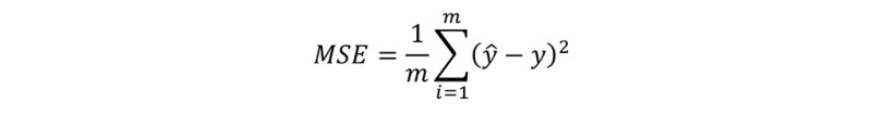
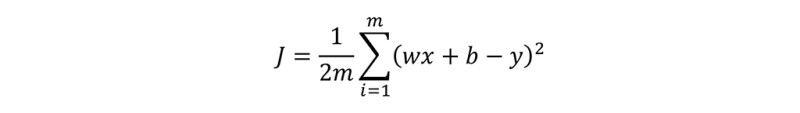
∑ indicates the sum of all values of SE. To make later calculations faster and neater, we divide the above equation by 2. This division by 2 reduces the amount of time needed to calculate large values of MSE. In regression problems (discussed later), MSE is denoted by J. So, the final equation, is shown below.
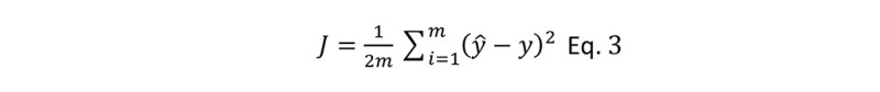
This J is called cost function. SE is the square error at one value of x while the cost function is the average of all SE.
Let’s find the cost function. In Table 2, I summarized all the values of SE. Sum all of them, which is 606, and ultimately, the cost function (J) is:
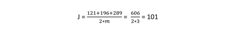
Now, think about it. If our predicted value (ŷ) is close to the real value (y), the cost function will be small. For example, if y is 11 and ŷ is 10.80 (pretty close), then SE will be 0.04. The smaller the SE, the smaller the cost function will be.
Therefore, the goal is to make the cost function (J) small. The smaller the J, the more accurate the model is. And that can only be possible if we find the best parameters (w and b). How to achieve it? Here comes Step 3.
Step 3
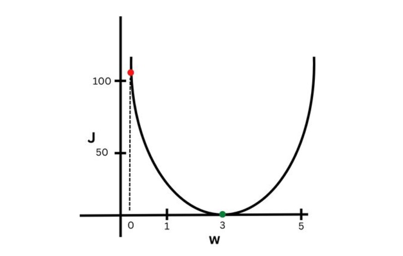
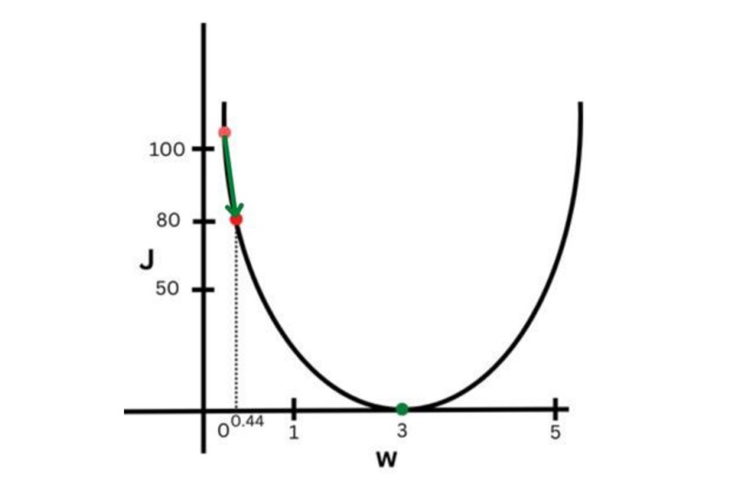
The third step is to minimize the cost function by finding the best values for the parameters. Let’s draw a curve between w and J (Fig. 2). We can draw a curve among w, b, and J, but it will be 3-D. For simplicity, I just draw for w and J. In Fig. 2, you can see the value of J = 101 (red dot) at w = 0.
Now we need to move the red dot closer to the green dot where J is near to zero. How do we do that? By taking small steps or jumps (Fig. 3).
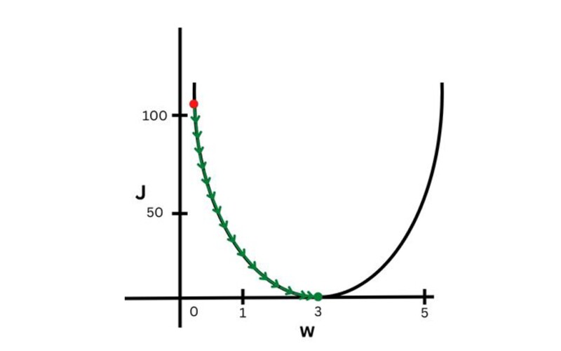
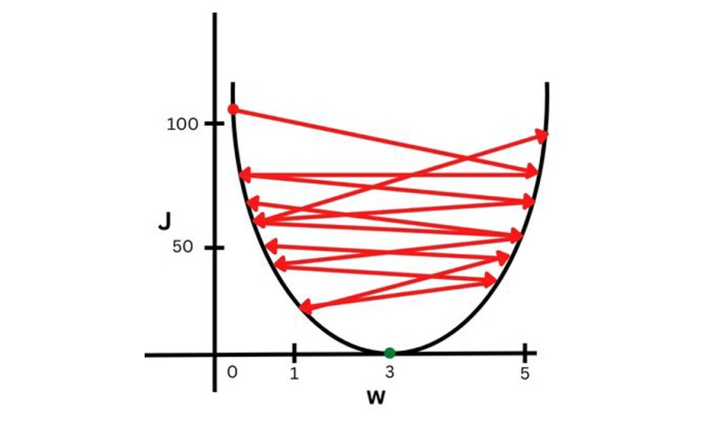
In Fig. 3, green arrows show the small jumps we need to take to reach from the red dot to the green dot. The step sizes of these small jumps are proportional to the learning rate, denoted by α (alpha). The smaller the alpha is, the smaller the jumps. However, if the learning rate is very large, then the cost function (J) will never converge (reach the minimum or zero). It will move back and forth as in Fig. 4. Therefore, the learning rate value is very important.
As previously mentioned, we need to take small jumps (green arrows in Fig. 3) to converge our cost function J. So, how do we do that?
Answer: Find the slope of the current point (red dot) and then adjust it slowly (small jumps). If you are familiar with calculus, you know that finding the slope means finding the derivative. If you didn’t study calculus, don’t worry, just remember that derivative and slope are the same thing. So, to find the slope of a line where the red dot is, we need to find the derivative of J with respect to w. We know from the above-mentioned Eq. 3 that J is:
From Eq. 2, put ŷ = wx + b in the above equation. So,
If you are familiar with calculus, you know derivative (technically, partial derivative) of the above equation with respect to w is:
And with respect to b is:

Note the difference. Derivative with respect to b doesn’t have the x term in the last part.
So far, so good. Let's review some basic concepts from high school mathematics. A horizontal line has a slope of zero, a line at 90° has an undefined slope, and lines between 0° to 89° or -91° to -180° have positive or negative values of slope. This is illustrated in Fig. 5.
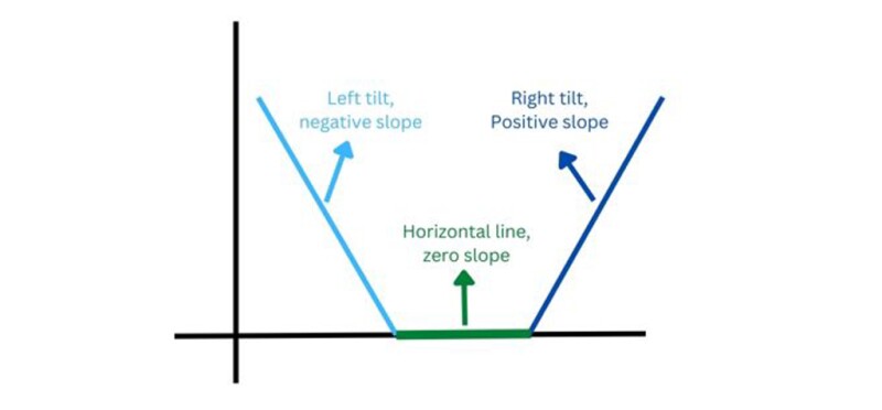
As shown in Fig. 5, I have drawn three lines. The green line is a horizontal line with a slope of zero. The blue line, which is tilted to the left, has a negative slope value. The cobalt blue line, which is tilted to the right, has a positive slope value. It's important to note that a straight line has the same slope at all points, while a curve has different slopes at different points.
In Fig. 3, the red dot represents a curve that is tilted to the left (negative slope) and the green dot represents a horizontal line (zero slope). To move from the red dot to the green dot, we need to increase the slope (from a negative value to zero). If the red dot were on a curve that was tilted to the right (positive slope), we would need to decrease the slope (from a positive value to zero). The procedure is the same in both cases.
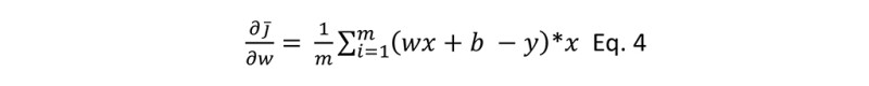
Let’s find out the value of slope with respect to w and b using Eq. 4 and Eq. 5.

I compiled all the values with respect to w and b in Tables 3 and 4, respectively. Remember that m is 3.

So, from above Table 3, we have a slope with respect to w (∂j/∂w) as -44. Now we have to make it zero or near zero (increasing). To increase the slope, we need to find the new value for w. Remember, we will achieve this by taking small jumps. Let’s set the small jump (α) value equal to 0.01. The formula for the new w (or updated w) after a small jump is:

Put all the values, w(current) = 0, α = 0.01, and (∂j/∂w) = -44
w(updated) = 0 – 0.01*(-44) = 0+0.44
w(updated) = 0.44
We successfully determined the new value for w after one small jump. Let’s do the same process for b.

The slope with respect to b (∂j/∂w) from above Table 4 is -14. Like w, we have to make it zero or near zero by taking small jumps. Put all the values, b(current) = 0, α = 0.01, and = -14 in Eq. 7.

b(updated) = 0 – 0.01*(-14) = 0+0.14
b(updated) = 0.14
Hence, we completed our first iteration (one small jump) and determined the new (updated) values for w and b. This third step is called gradient descent (finding the derivatives) and then updating the gradient descent (determining the new values for parameters). Let’s revise what we have done so far.
- Initialize parameters: by setting w = b = 0.
- Find the cost function: first, find the square error, then sum all the SE and finally determine the J.
- Find and update the gradient descent: derivative of cost function and then update the values of w and b.
Now we have new values for w and b, 0.44 and 0.14 respectively, after one small jump. So, repeat steps 2 and 3 to get new values for w and b (updated one more time), after one more small jump (second jump). Remember that m is 3. I summarized the step 2 calculation in Table 5.

Here, after first jump, cost function is 80.81 which is less than the previous cost function (101). See Fig. 6.
Now, repeat Step 3 (finding and updating gradient descent).
First, find out the value of slope with respect to w and b using Eq. 4 and Eq. 5.
We compile all the values with respect to w and b in Table 6 and Table 7.
Table 6 (for w)

Now it is time to jump, one more time. The formula for updated w after one more small jump is the same as the previous one:
But this time w(current) = 0.44, (∂j/∂w) = -39.42 and α is same as previous one, 0.01.
w(updated) = 0.44 – 0.01*(-39.42) = 0.44+0.3942
w(updated) = 0.83
Table 7 (for b)

Now it is time to jump, again. Same formula but b(current) = 0.14, (∂j/∂b) = -12.54, and you know α = 0.01.
b(updated) = 0.14 – 0.01*(-12.54) = 0.14+0.1254
b(updated) = 0.26
Notice that after the completion of the second iteration, the new values of w and b, 0.83 and 0.26, respectively, have increased compared to the previous w and b, 0.44 and 0.14. We need to keep taking small jumps until we get w and b equal to (or near to) 3 and 5, respectively, as we have y = 3x + 5 (Eq. 1). I used Python for 1,000 and 5,000 iterations and summarize the values in Table 8.
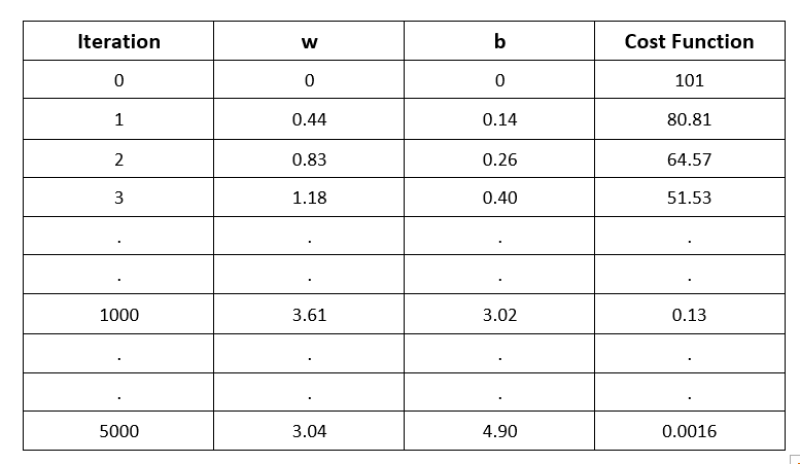
Notice that at the 5,000th iteration, the value of w is 3.04 which is close to 3, and that of b is 4.90 (close to 5). Also, it would be noticed that the cost is decreasing with every iteration.
Yeah, that’s it. You have successfully trained your first machine learning model (linear regression model). But wait a minute. This is a basic model while real-life problems are complex. So, wait for further parts in this series.
Let’s add, in passing, some more fun. We used both input and output to train our model. This type of machine learning (having both input and output) is called supervised learning. On the other hand, in unsupervised learning, we have just input (no output), and the machine learning model's task is to find the patterns within the data. Moreover, in this case, output was a numerical value (from -infinity to +infinity). This type of problem is called a regression problem. While classification problems have a limited set of output options, such as binary outcomes (cat or dog, oil or gas) or multiple categories (cat, dog, or fish; oil, gas, or water).
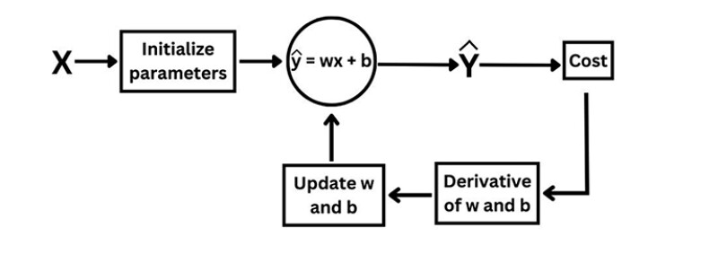
Up to this point, you know what is cost function and gradient descent. We use ŷ = wx + b which is called a linear activation function. In the first step, we initialized parameters (w and b) with zero, in the second step we determined the cost function. This is called feed forward propagation. In the third step (gradient descent), we went back to determine the derivative (slope) and then updated the values of w and b. This is called feed backward propagation. So, machine learning is the combination of both, and named as feed forward back propagation. See Fig. 7 for a visual representation:
Let’s summarize the steps of this basic machine learning model:
- Initialize parameters with zero
- Find the cost function:
- Square error (SE)
- Mean square error (MSE)
- Find and update the gradient descent:
- Derivatives of w and b
- Update the values of w and b
- Repeat Steps 2 and 3.
For a hands-on experience, click here to check the Python code of this basic model. At the end of the code, I have replaced the values of x and y with real-world examples of porosity and permeability.
Feel free to try it with your own data. If the cost function continues to decrease at each iteration, it indicates that your model implementation is correct.
Congratulations! You are now familiar with:
- Supervised learning
- Unsupervised learning
- Regression problem
- Classification problem
- Feed forward propagation
- Feed backward propagation
- Feed forward back propagation
- Linear activation function
- Cost function
- Gradient descent.
Read part 2 and part 3.
