
The flow-network-based models are among those promising solutions that are under rapid development, where minimum geological information is necessary to build them. This article focuses on the introduction of one of the flow-network-based models called GPSNet that has growing popularity in the literature and shows promising results during our proof-of-concept applications.
Introduction to Flow-Network Models
Decision-making in modern reservoir management increasingly relies on predictions from simulation models. These models represent geological features, such as faults, channels, and rock and fluid properties through grid blocks. However, a 3D full-physics geo-cellular simulation model is not always the most fit-for-purpose solution.
Firstly, building and maintaining a full-physics model for reservoir simulation is both time-consuming and expensive since it requires input data from multiple disciplines. In addition, the model can be computationally prohibitive to calibrate to field data measurements which typically require hundreds of simulations. This is especially true for mature reservoirs with hundreds of wells and decades of production history.
The General Purpose Simulator-Powered Network (GPSNet) is a physics-based data-driven flow-network model implemented by Ren et al. (2019) following the idea of Lutidze and Younis (2018) and later extended by Wang et al. (2021, 2022) to mature waterflood and steamflood cases.
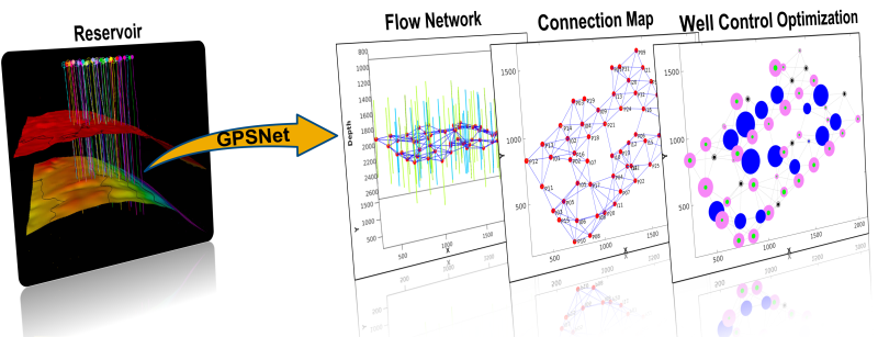
As illustrated in Fig. 1, it first generates a flow-network model that consists of interwell connections following the well-completion information, and the full-physics flow equations are numerically solved on these connections. By doing so, GPSNet removes many limitations of other flow-network-based models that entirely or partially rely on analytic/empirical solutions and simple material balance relation.
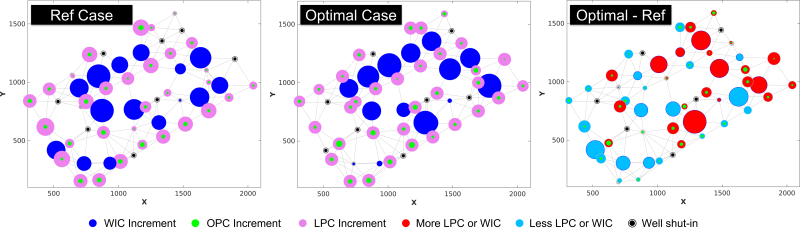
The rightmost figure displays a bubble plot summarizing a well-control-optimization outcome, where the well cumulative injection/production are shown. The use of a commercial simulator makes it applicable to different field development strategies varying from secondary waterflood to tertiary enhanced oil recovery processes. It serves as an ideal surrogate model for both fast and reliable decision-making in reservoir management.
How Is the Flow Network Created in GPSNet?
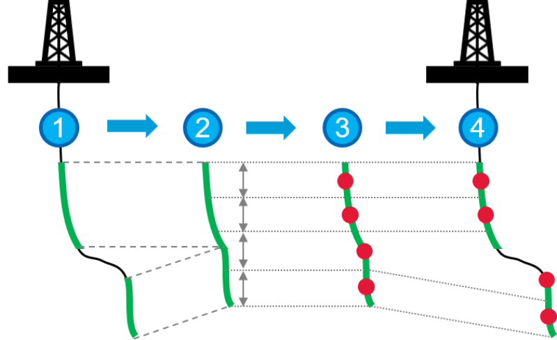
To build a GPSNet model, one needs to first construct a flow network following the well completions, the minimal geological information requested in GPSNet. Fig. 2 illustrates the steps to discretize the discontinuous completions (green curves) along a wellbore with four well points (red dots). Each perforated and completed portion will be added up, then the sum will be evenly divided into pieces and the well points will be placed at the center of each portion, and finally the well points will be mapped back to the well trajectory. Unless there is a strong gravity/layering effect, it is recommended to use only one point per well whenever possible for a simple flow network.
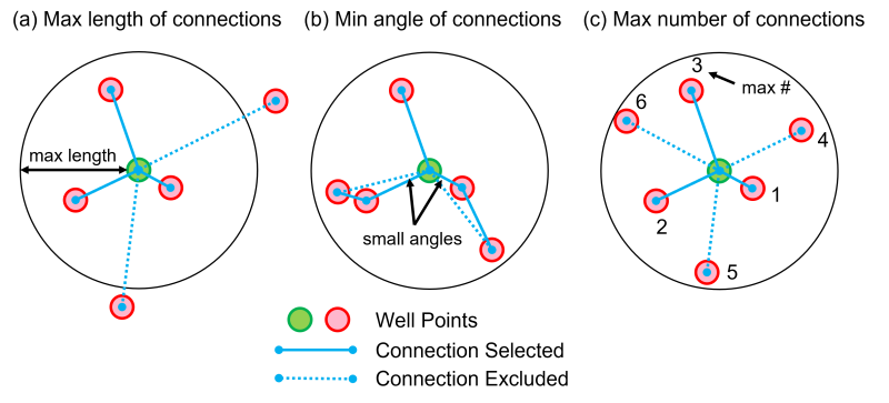
Once the well completions have been discretized, the next step is to create connections that link the well pairs through the completions. Our best practice is to create the preliminary flow network using the parameters shown in Fig. 3.
- Maximum length between connected wells
- Minimum angle of connections that emit from the same well
- Maximum number of connections per well
For each well point under investigation (green circles), connections shorter than the maximum length (solid lines) will be created. If the angle of two connections is less than the minimum angle, eliminate the longer one. Then, exclude the longest connections if the total number of connections exceeds the maximum number. Finally, quality check the created flow network with field engineers and geologists and adjust before history matching.
How To Create a GPSNet Model
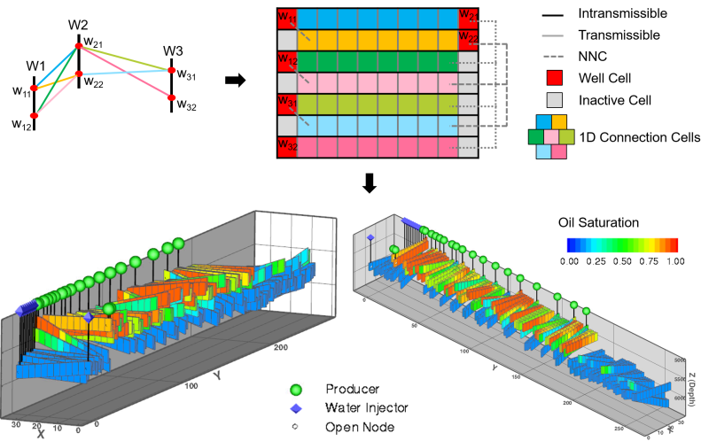
To build a GPSNet model for fields with thin formations and limited gravity effects, one needs to map the flow network to a standard grid system for the simulation process. Fig. 4 illustrates the mapping procedure from the flow network to a series of 1D discretized connections. The portion of the flow network displayed on top left of the figure contains three wells with two well points each and seven connections. Spatial discretization is then performed, and the portion of the flow network is mapped to a series of 1D discretized connections, one connection per row, as the top-right plot depicts. All the grid cells along the seven connections, including the well cells, follow the same color-coding with the flow network on the top left. Notice the intransmissible barriers (black solid lines), transmissible cell interfaces (gray solid lines) and non-neighbor connections (NNC, gray dashed lines) are marked differently. The bottom plot displays the initial oil-saturation distribution used in the reservoir simulation after phase equilibrium.
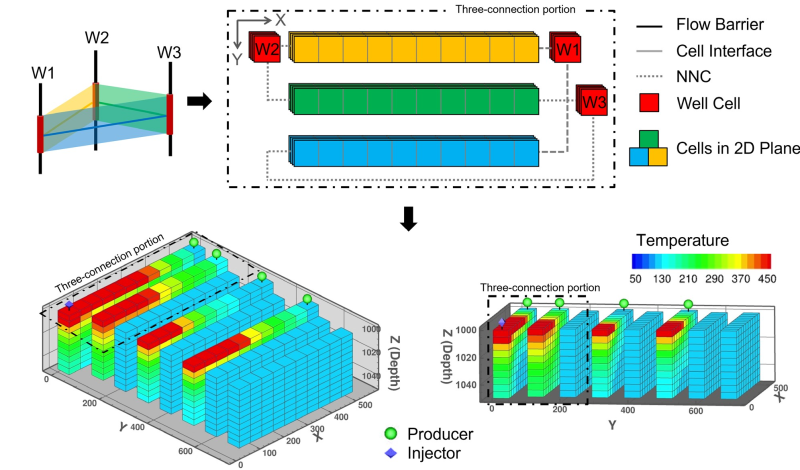
For fields with strong gravity effects, like steamflood or waterflood in thick formations, it is challenging to capture concurrent vertical and horizontal flows through 1D connections. Instead, the reservoir is discretized into a series of 2D connections (x-z planes) between well completions as shown in Fig. 5. These connection planes, designed as vertical slices, capture the main areal/vertical flow paths in the reservoir.
Once the GPSNet model is established, the grid properties of each connection are then interpreted with historical data. The following is a list of key uncertainty parameters of GPSNet models that need interpretation from production data:
- Relative permeability model parameters
- Capillary pressure
- Water/oil contact depth
- Initial reservoir pressure/temperature
- Fluid pressure/volume/temperature relationship
- Flow/thermal transmissibility multipliers
- Heat loss, aquifer, gas cap
- Rock/pore volume multipliers
- Injector/producer well indexes
The best-matched models are then selected for optimization. We have already demonstrated the effectiveness through several proof-of-concept applications.
GPSNet Application Results
Once a GPSNet model is created for a field, we will need to train its accuracy to match historical field/well performance. Considering the historical data available, the history-matching targets are usually set to be field liquid/oil production cumulative (FLPC/FOPC), well liquid/oil production cumulative (LPC/OPC), and bottomhole pressure/temperature (BHP/BHT). The history-matching process is designed to be an iterative process with a five-step hierarchical structure, and each step matches more historical data than the previous one as illustrated in Fig. 6.
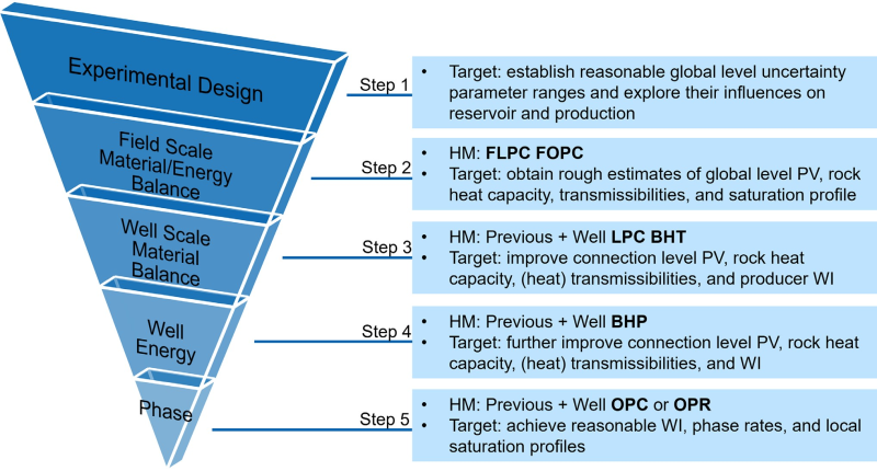
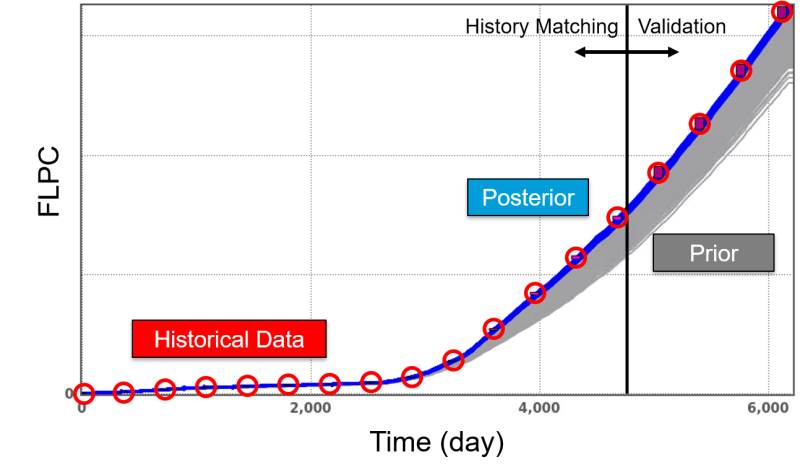
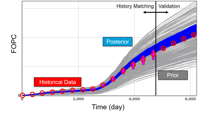
Fig. 7 shows the field-level results in Step 5 of a waterflooded diatomite reservoir, where a portion of historical data was preserved to validate the reliability of the GPSNet model. Both FLPC and FOPC match closely with historical data in the posterior ensemble (blue curves), including the prediction period. It is worth mentioning that each simulation case costs approximately 50 seconds on a single core. Steps 1 through 5 required a single day to complete, which includes result analysis and 2,700 GPSNet simulation runs.
After that, we used a historically matched GPSNet model for injection-rate reallocation optimization to maximize economics under field/well constraints. Fig. 8 compares water injection cumulative (WIC), OPC, and LPC during the prediction period, and the circle area is proportional to the fluid volume. These recommendations could be helpful to reservoir engineers when designing the injection plans and well schedules.
Conclusions
The GPSNet model combines flow-network model with a commercial simulator such that it can model complex physical processes while still be computationally efficient for history matching and optimization studies. Furthermore, complex well schedules and various well/field level constraints can be easily realized in GPSNet just like regular simulation models.
Unlike traditional simulation that relies on a detailed characterization of geological models, the GPSNet model only requires well volumetric production/injection data and its approximate trajectory and can be generated and updated rapidly. In addition, GPSNet also runs much faster than a full-fidelity model due to having fewer grid blocks in the model. The key features of the GPSNet models are summarized below.
- Data-driven and physics-based—no need for full 3D models and very fast with full physics
- Adaptive to data quality and available reservoir information
- Numerical solution based on completion-wise connections and trained with historical data
- Validated for waterflood and steamflood cases.
Thus, it can serve as a promising surrogate for the full-fidelity reservoir simulation models to achieve a fast and reliable decision-making process.
For Further Reading
Proxy Reservoir Simulation Model for IOR Operations by G. Lutidze and R. Younis, University of Tulsa.
SPE 193855 Implementation of Physics-Based Data-Driven Models With a Commercial Simulator by G. Ren, University of Tulsa; and J. He and Z. Wang, Chevron Corporation, et al.
SPE 200772 Fast History Matching and Optimization Using a Novel Physics-Based Data-Driven Model: An Application to a Diatomite Reservoir by Z. Wang and J. He, Chevron ETC; and W. Milliken, Chevron Corporation.
SPE 209611 Fast History Matching and Robust Optimization Using a Novel Physics-Based Data-Driven Flow-Network Model: An Application to a Steamflood Sector Model by Z. Wang and X. Guan, Chevron Technical Center; and W. Milliken, Chevron North America Exploration and Production, et al.
