
The age-old question of which came first, the chicken or the egg, remains unanswered. Similarly, the oil and gas industry utilizes existing models from other branches of science—modifying, simplifying, complicating, customizing, and configuring them to achieve new objectives. While reusing pre-existing models is a common scientific practice, the petroleum industry represents the pinnacle of this art form.
This article introduces ten crucial equations essential to various aspects of the upstream petroleum industry. These equations play a fundamental role in understanding how science drives the exploration and production processes of oil and gas operations. This list is not exhaustive but serves as a primer to the simultaneous simplicity and complexity inherent in the petroleum industry.
1. Bragg’s Law
Reliability is the bedrock of the exploration phase, playing a pivotal role in minimizing the time-to-market of a reservoir. The more accurate the information gleaned from exploration data, the quicker we can reach the reservoir and evaluate its exploitability.
One of the most important geophysics laws that aids us in this endeavor is Bragg’s Law. Developed by father and son duo William Henry Bragg and his son William Lawrence Bragg in 1913, this formula studies the interference phenomenon of multiple reflections in crystals, offering us a practical tool for efficient exploration.
Bragg’s Law is synthesized in the formula:

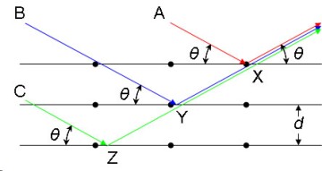
Where λ is the wavelength [m], d is the distance between 2 consecutive crystalline planes [m], θ is the angle between the reflected wave and crystalline plane, and n is the diffraction order.
In oil and gas exploration, seismic waves act as the primary tool. By applying Bragg's Law principles, particularly the Law of Superposition and the Principle of Original Horizontality, geologists can interpret the complex signals received by geophones. This allows them to reconstruct the subsurface structure, a crucial step in identifying potential oil and gas reserves.
2. Hubbert Equation/Curve
The Hubbert Equation is often used to model the temporal evolution of oil production from an exhaustible mineral/fossil source. The equation was developed by geophysicist M. King Hubbert who predicted in 1956 that fossil fuel production in a given region over time would follow a roughly bell-shaped curve. His creation of the Hubbert Equation/Curve was designed to estimate future production using past observed discoveries.
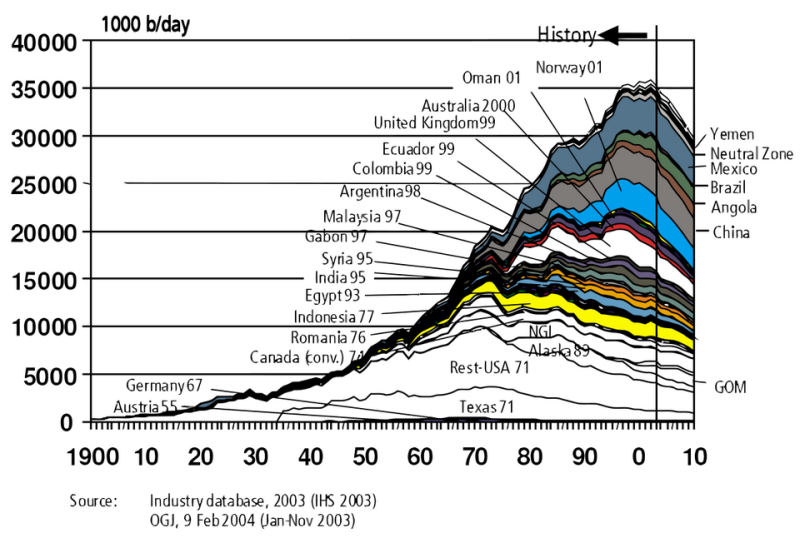
The main equation is similar to the one of a Gauss bell distribution:

Where P(t) is the oil production [bbl] for year t [y], Qm is the estimation of ultimate oil production [bbl], w is an inverse decay time [y-1], τ is the year [y] at which production peaks (Claerbout and Muir, 2008).
3. Material Balance
Oil production can be monitored and, ideally, predicted using a straightforward material balance approach. Central to this is the Oil Material Balance equation:

Here Np is the cumulative production [bbl], OOIP is the original oil in place [bbl], f is reservoir porosity [-], Pi is the initial reservoir pressure [psi], Pwf is the flowing bottom-hole pressure [psi], m is the isochoric compressibility [psi-1], ΔP is the variation of bottomhole pressure [psi] in time and Np0 is the cumulative production [bbl] related to the previous time interval. This equation can be derived by combining the definitions of OOIP and compressibility.
Time dependency is introduced by Np0 (since this equation can be applied to a specific time interval) and Δp (that is the variation of flowing bottomhole pressure in time). The latter takes into account the variation of reservoir pressure due to depletion.
4. Darcy’s Law
Who would have thought an equation originally formulated for hydrogeology would find such diverse applications within the oil industry? Darcy’s Law is expressed as:

Where q is flow rate [m3/s], k is porous medium permeability [m2], μ is fluid viscosity [Pa∙s] and p is pressure gradient [Pa*m].
The pressure gradient consider pressure drops along the porous medium due to frictions. In other word, it describes the driving force of the flow. It should not be confused with the “hydraulic gradient”, which is commonly used to describe the density of the fluid.
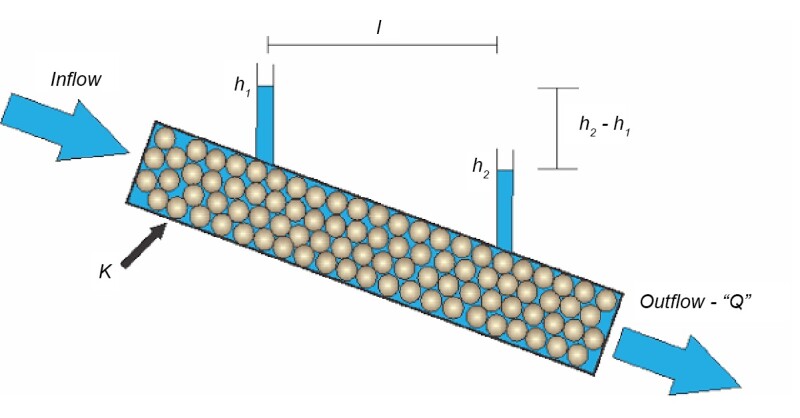
This law was derived by French engineer Henry Darcy in 1856 from his experiments on flow through sand beds which comes with certain constraints in its original form.
● It assumes the porous media to be homogeneous, isotropic, and fully saturated with the fluid.
● It considers the flow across the pores to be one-dimensional and laminar.
● It assumes the fluid to be incompressible.
Darcy’s Law represents a fundamental base for reservoir studies, and it has been subsequently generalized for multiphase flow and inhomogeneous reservoirs. Dynamic modeling, history matching, reservoir management, and production forecasts are all based on this simple but robust equation.
5. Stevin’s Law in Field Units
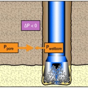
Once geophysicists have worked their magic with Bragg’s Law, it is the turn of professionals that must practically reach the oil. Stevin’s Law states that the pressure at any point within a fluid at rest (of a certain density) depends only on the depth of that point: undersea, pressure increases according to this law. Drilling the first well is something like making a bet. It is expected to find porous rocks filled with fluid at a certain depth.
This law is used for the calculation of the pressure exerted by the mud column in the wellbore hole, or, reverting it, to calculate the density of the mud to balance a certain pressure at a certain depth.
However, as well as the drilling bit digging into the subsurface, the pressure encountered grows faster. The drilling mud helps drillers to prevent any blowout, keeping fluids in the formation. This is thanks to Stevin’s Law, adapted to be used in field units:

Where P is the pressure exerted by the column of fluid [psi], ρ is the mud density [ppg], and TVD is the vertical depth [ft]. The coefficient 0.052 includes not only the gravitational acceleration (g), but also the conversion from SI units to field ones.
Interestingly, the above equation is just a customized and unit-specific version of Pascal’s Law.
6. Annular Capacity
The annular volume of a well is an essential parameter which provides value from basic depth correlation to well integrity and well control. Well integrity plays a crucial role both in the drilling and production phases. The void space between tubing and casing (annulus) can be cleverly utilized to detect tubing or casing leakages by filling it with a fluid (e.g., packer fluid) and constantly monitoring its pressure. Even though the volume calculation is simply a cylinder, a simplified equation as shown below makes it easier for the driller to perform calculations in the field.
The volume between any two pipes is given by the annular capacity, calculated as:

Where V is the volume per length [bbl/ft], OD is the diameter of the outside wall of the annulus [in], ID is the diameter of the inside wall of the annulus [in], 1029.4 is a constant derived by unit conversion.
For calculating the capacity of a single pipe, simply replace the OD with the internal diameter of the pipe and the ID can be set as 0. This equation can be rearranged in various ways to suit differing scenarios.
7. Inflow Performance Relationship (IPR): Vogel’s Equation
Monitoring and controlling well performance is crucial for forecasting oil and gas production and ensuring the well operates at its peak potential. In this context, the Inflow Performance Relationship (IPR) curve plays a vital role. It establishes a relationship between the well's bottomhole pressure and the produced flow rate.
Since the IPR curve depends on the fluid composition (oil, gas, and water ratios), Vogel's Equation is presented here as an example for oil and associated gas production:

Where qo is the oil flow rate [bbl/d], Pwf is the well bottomhole pressure [psi], Pres is the average reservoir pressure [psi].
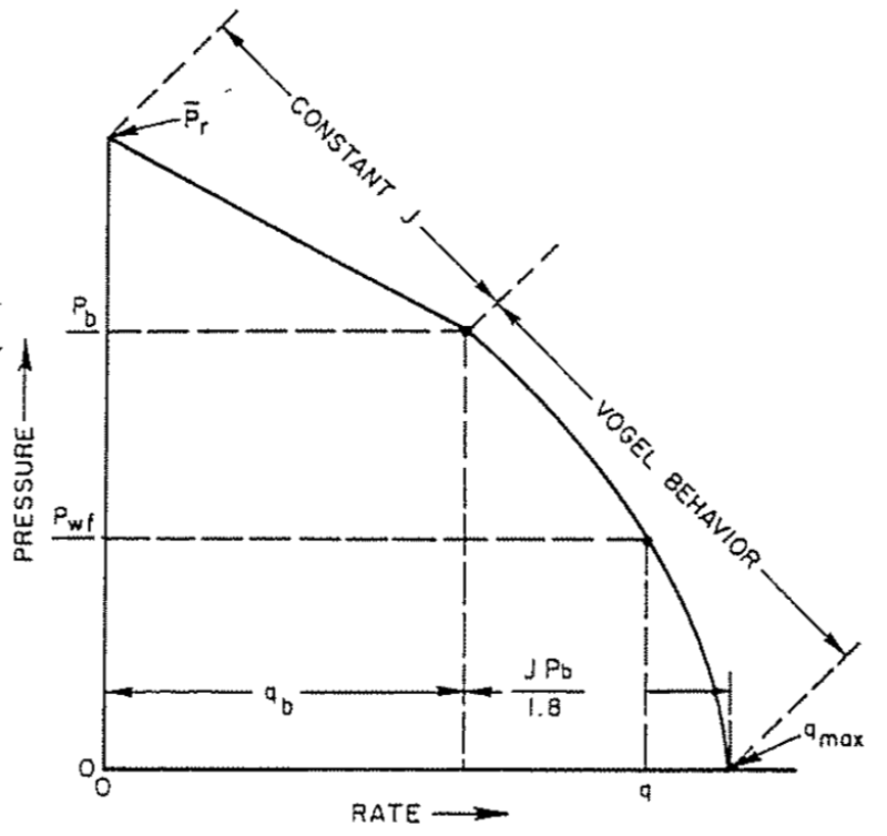
Vogel’s IPR relationship is a powerful tool in two-phase flow: for pressure above the bubble point, pressure and flow rate are linearly bonded according to the productivity index (J) definition; for pressure below the bubble point, the Vogel behavior better represents this relationship.
8. Bernoulli’s and Poiseulle’s Equations
In the oil and gas industry, two key equations govern fluid behavior: Bernoulli's Equation and the Hagen-Poiseuille Equation (often referred to as the Poiseuille Equation).
- Bernoulli's Equation relates pressure, height, and flow rate based on the principle of energy conservation.
- The Poiseuille Equation describes the pressure drop within a pipe due to the fluid's flow rate and viscosity.
These equations are expressed as:

Where v is fluid velocity [m/s], g is the gravitational acceleration [m/s2], z is the height [m], p is the pressure [Pa], ρ is the density [kg/m3], μ is the viscosity [Pa s], L is pipe length [m], R is the pipe radius [m] and q is the flow rate [m3/s].
Since Stevin’s Law is valid only for hydrostatic cases, Bernoulli’s and Hagen-Poiseuille's equations are utilized for fluid dynamics, in particular, incompressible and Newtonian fluid in laminar flow. These assumptions might not be always respected in describing oil behavior, because it is not Newtonian at all and not applicable to light oil and gases, due to high compressibility and turbulence. For this reason, they are only the basis for further modeling in the oil industry.
9. Real Gas Equation of State
Accurately modeling gas behavior is more complex than modeling liquids due to their compressibility, lighter weight, lower viscosity, and ability to mix with other gases in any proportion. Since oil, associated and nonassociated gases comprise hundreds of compounds, precise modeling of their thermodynamic properties is crucial.
One of the most widely used tools for this purpose is an Equation of State (EoS). An EoS relates the pressure, volume, and temperature of a gas. Among the various EoS, the Soave-Redlich-Kwong (SRK) equation, a cubic equation, is particularly popular:


Where P is the pressure [Pa], T is the temperature [K], Ṽ is the molar volume [m3/mol], ω is the acentric factor [Pa], Tc is the critical temperature [K], Pc is the critical pressure [Pa], Tr is the reduced temperature [-] and R is the universal gas constant [Pa∙m3/(mol∙K)].
The SRK equation is a refinement of the existing Redlich-Kwong (RK) Equation. Giorgio Soave proposed adding the dependency of α(T) by the square root of Tr to improve vapor pressure prediction for hydrocarbons (Soave, 1972).
10. Oil and Gas Property Evaluation
The economics of oil and gas operations can be quite complex. Once a field has been discovered and reserves estimated, companies may combine resources to form a joint venture that shares the production risks. However, assessing the value of producing properties can be exceedingly challenging once the field enters production. The equation guiding this evaluation is as follows:

Here P is the current value of the cumulative net cash flow stream [$], N is the revenue interest [-], R is the reserves estimation [bbl], W is the wellhead price [$/bbl], T are the wellhead taxes [$], C are the operating costs [$], F are the federal income taxes [$], and I are the investments made [$].
While the equation appears quite simple, each variable harbors uncertainties that must be estimated with great care. These uncertainties stem from factors like geology, engineering, legal issues, political climate, and economic fluctuations inherent in oil and gas operations (Rose, 2012).
For Further Reading
X-Rays and Crystal Structure by W.H Bragg and W.L. Bragg.
SPE 209945 A New Real Time Prediction of Equivalent Circulation Density From Drilling Surface Parameters Without Using PWD Tool by M.M. Al-Rubaii, Saudi Aramco.
M. King Hubbert, 86, Geologist; Research Changed Oil Production by A.A. Narvaez, The New York Times.
Hubbert Math by J. Claerbout and F. Muir.
Equilibrium Constants From a Modified Redlich-Kwong Equation of State by G. Soave, Chemical Engineering Science.
Fundamental Economic Equations for Oil and Gas Property Evaluation by P. Rose.
Peak Oil Theory by C. O’Leary, Encyclopedia Britannica.
Pioneering Geophysicist’s Theory of Peak Oil Still Debated by T. Sumner, ScienceNews.
