LSTM for Production: Part 1

Accurate production forecasting plays a pivotal role in understanding and effectively developing reservoirs. Numerous research shows that machine learning could be used to achieve fast and precise production predictions. In this three-part article, we use long short-term memory (LSTM), a machine learning technique, to predict oil, gas, and water production using real field data. This first part discusses the mathematics behind the LSTM and part two and three focus on its practical implementation.

Recurrent neural network (RNN) and its variants, namely LSTM and gated recurrent unit (GRU), are specifically tailored for time-dependent data. They retain long-term dependencies while maintaining accuracy across varying time scales. The LSTM and GRU networks are ideal for processing long sequential data because of the unique memory cell and gating mechanism, that stores and retrieves information over time. This makes them suitable for handling forecasting problems that require consideration of past and present data. Even a bidirectional (two-way) network can take context from both, past and future, much like Loki, “adopted brother” of Thor Odinson. In this article, our primary focus lies on LSTM. However, before delving into its mathematics, we first make a short digression to introduce the concept of simple RNN.

The recurrent neural network is the repeated use of a single cell. Fig. 1 describes the operations of that single cell for a single time step.

All figures reproduced with permission from DeepLearning.AI.

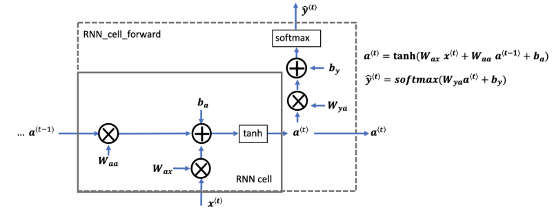
This RNN cell takes the current input, 𝑥^<𝑡>, and the previous hidden state containing information from the past, 𝑎^<t-1>, and outputs the current hidden state 𝑎^<𝑡>. This current hidden state is then given to the next time step (of the same RNN cell) and also used to predict 𝑦̂^<𝑡>. For the first-time step, where no previous hidden state exists, 𝑎^<0> is initialized to zeros. The mathematical equations are given on the right side of Fig. 1. You can see the use of the “softmax” activation function for 𝑦̂^<𝑡> but we can use any other activation function as well, depending on the problem at hand.

Trainable parameters are initialized randomly. As illustrated in Fig. 1, these parameters include:

• W_ax: The weight matrix multiplying the input
  
• W_aa: The weight matrix multiplying the previous hidden state
  
• W_ya: The weight matrix that connects the current hidden state to the output
  
• b_a: Bias term
  
• b_y: Bias term linking the hidden state to the output

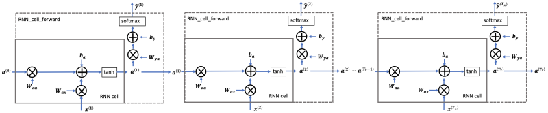
In the forward pass of the RNN, a single cell (Fig. 1) is repeated multiple times. For instance, if the input is 10-time steps long, we will re-use that RNN cell 10 times. At each time step, the cell takes two inputs: the hidden state from the previous cell (𝑎^<𝑡-1>) and the current time step's input data, (𝑥^<𝑡>). It has two outputs at each time step: a hidden state (𝑎^<𝑡>) and a prediction (y^<𝑡>). The weights and biases (𝑊_𝑎𝑎, 𝑊_𝑎𝑥, 𝑏_𝑎, 𝑊_𝑎𝑦, 𝑏_𝑦) are re-used at each time step. Fig. 2 shows the forward pass of RNN (a single cell is used multiple times).

Though RNN is relatively robust, it still suffers from vanishing gradient for long piece of information. Therefore, we will build a more sophisticated model, the LSTM, which is better at addressing vanishing gradient and remembering a piece of information for many time steps.

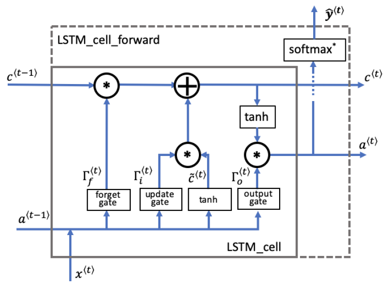
The LSTM is similar to RNN in that they both use hidden states to pass along information, but LSTM also uses an additional component named cell state, which is like a long-term memory, to help deal with the issue of vanishing gradients. An LSTM cell consists of a cell state (c) for long-term memory and a hidden state (𝑎) for short-term memory, along with three gates (forget gate, update gate, and output gate) that control the flow of information and constantly update the relevancy of its inputs.

A forget gate (𝚪𝑓^<t>) decides which information to retain or forget. An update gate (𝚪𝑖^<t>) decides on what new information to add, and what information to throw away. And an output gate (𝚪𝑜^<t>) decides what information gets sent as the output of the time step. Detailed explanations of these gates follow below.

Fig. 3 shows the operations of a single LSTM cell for a single time step.

Mathematics Behind Gates

Forget Gate 𝚪f^<t>

The forget gate equation is:

 

Where W_𝑓 and b_𝑓 (forget gate weight and forget gate bias) are learnable parameters, initialized randomly, 𝑎^<t-1> is a hidden state of the previous time step, 𝑥^<𝑡> is the input of the current time step, and 𝜎 shows the use of sigmoid function.

The W_f contains weights that govern the forget gate's behavior. The previous time step's hidden state (𝑎^<t-1>) and current time step's input (𝑥^<𝑡>) are concatenated together and multiplied by W_f. A sigmoid function is used to make each of the gate tensor's values range from 0 to 1.

The forget gate has the same dimensions as the previous cell state c^<t-1>. This means that these two can be multiplied together, element-wise (component-wise). Multiplying the forget gate with previous cell state (𝚪𝑓^{<t> *}c^<t-1>) is like applying a mask over the previous cell state. If a single value in is 0 or close to 0, then the product is close to 0. This keeps the information stored in the corresponding unit in c^<t-1> from being remembered for the next time step. In other words, the LSTM will "forget" the stored state in the previous cell state. On the other hand, if a value is close to 1, then the product is close to the original value in the previous cell state. This means that LSTM will keep the information from the corresponding unit of c^<t-1>, to be used in the next time step.

Candidate Value 𝐜̃^⟨𝐭⟩
The candidate value equation is:

 

The candidate value (𝐜̃^⟨𝐭⟩) is a tensor containing information from the current time step that may or may not be stored in the current cell state c^<t>, depending on the value of update gate. The use of tanh function produces values between -1 and 1. The tilde "~" is used to differentiate the candidate from the cell state c^<t>.

Update Gate  𝚪𝒊^<𝐭>
The update gate equation is:

 

Notice that the subscript "i" is used and not "u" to denote "update", to follow the convention used in the literature.

The update gate decides what aspects of the candidate value (𝑐̃^⟨𝑡⟩) to add to the cell state c^<t>. The use of sigmoid produces values between 0 and 1. When its value is close to 1, it allows the candidate value to be passed onto the cell state c^<t>. But when its value is close to 0, it prevents the corresponding value in the candidate from being passed onto the cell state. The update gate is multiplied element-wise with the candidate (𝚪𝑖^⟨𝑡⟩∗ 𝑐̃^⟨𝑡⟩), and this product is then used to calculate the cell state c^<t>.

Cell State c^<t>
The cell state equation is:

 

The cell state is the long-term memory that captures information over long sequences and time steps. The new cell state c^<t> is a combination of the previous cell state c^<t-1> and the candidate value (which contains information from the current time step). The previous cell state c^<t-1> is adjusted (weighted) by the forget gate 𝚪𝑓^<t> and the candidate value is adjusted (weighted) by the update gate 𝚪𝒊^<𝐭>_.

Output Gate 𝚪𝒐^<𝐭>
The output gate equation is:

 

The output gate decides what information gets sent as the prediction (output) of the time step. Like the other gates, it also uses the sigmoid activation function that makes the gate range from 0 to 1. If its value is close to zero, it holds the information flow, and the output (y^<𝑡>) is predominantly influenced by the hidden state (a^<t−1>). On the other side, if its value is close to 1, it allows the information from the current input (x^<t>) to strongly influence the output.

Hidden State a^<t>
The hidden state equation is:

 

The hidden state is the short-term memory that captures information relevant to the current time step and the recent past. It is determined by the cell state c^<t> in combination with the output gate 𝚪𝒐^<𝐭>. The cell state is passed through the tanh activation function to rescale values between -1 and 1. The output gate acts like a "mask" that either preserves the values of tanh(c^<t>) or keeps those values from being included in the hidden state a^<t>. The hidden state is used for the prediction y^<𝑡> and also influences the output of the three gates of the next time step.

Prediction y^<𝑡>
The equation of prediction depends on the use of activation function. As alluded to above, we can use any activation function we want, suitable for a given problem. Fig. 3 above shows the softmax activation function, so, the equation of the prediction for the current time step is:

 

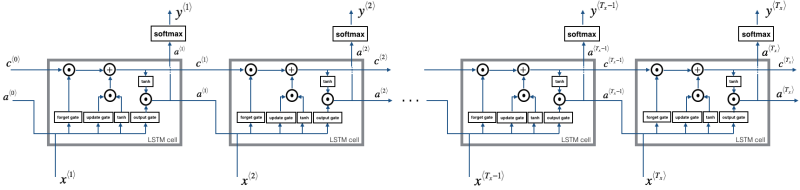
Similar to RNN, LSTM is a repetition of the LSTM cell (Fig. 3). If the input is 10-time steps long, then we will re-use the LSTM cell 10 times. Each cell takes three inputs at each time step: the previous hidden state (𝑎^⟨𝑡-1⟩), the previous cell state (c^<t-1>), and the current time step input data (𝑥^<𝑡>). It has three outputs at each time step: a hidden state (𝑎^⟨𝑡⟩), a cell state (c^<t>), and a prediction (y^<𝑡>). All the weights and biases are re-used at each time step. And, as we know that for the first-time step, there are no previous hidden state and cell state, so, 𝑎^⟨0⟩ and c^<0> are typically initialized as zeros. Fig. 4 shows the forward pass of LSTM (a single cell is used multiple times).

So far, we have seen the forward pass of LSTM. When using deep learning frameworks like TensorFlow or PyTorch, implementing the forward pass is sufficient to build your model. The framework will take care of the backward pass, that is taking the derivatives with respect to the cost to update the parameters. So most deep learning engineers do not need to bother with the details of the backward pass. If, however, you are curious and want to see the equations of backprop, they're briefly presented for your viewing pleasure below.

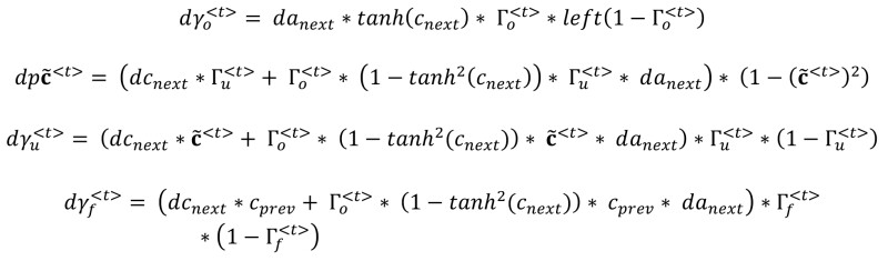
Gate Derivatives

 

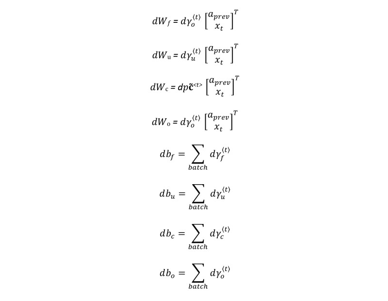
Parameter Derivatives

 

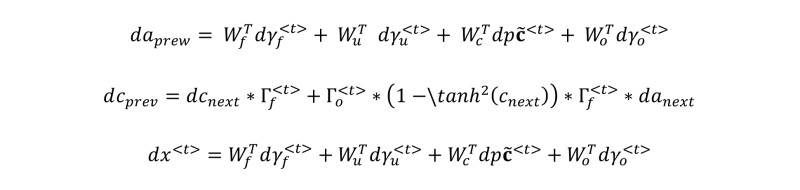
Memory and Input Derivatives

 

Feel free to derive all these equations from forward pass, if you are an expert in calculus. If you are not, it is okay not to understand all these. “Hail [TensorFlow]!”

In the next part,we will use the actual oil field data and TensorFlow to see LSTM in action. See you there.

Read Part 2 here.

Read Part 3 here.