
Welcome to the second part of our LSTM for production series. In the first part, we delved into the mathematics behind LSTM, and we are now ready to put all these into action. In this part, we will dive into practical example by using the production data of the Equinor’s Volve data set, a publicly available subsurface data set. We will train three separate univariate models to predict oil, gas, and water production. You can see the TensorFlow code here. I encourage you to open the link in a new window and read side by side of this article.
The Vovle dataset has around 40,000 files, including:
- Geophysical data, including interpretations
- Geo-Science Archive
- Production data
- Report
- Static models and dynamic simulations
- Seismic data
- Well logs
- Well technical data
- Realtime drilling data
To optimize model performance, it is imperative to extract all the relevant features from this wealth of data. This involves both spatial (static) and temporal (dynamic) data. For instance, extracting features from the Surface Operational Conditions, Details of all Wells Architecture, Well Logs, Core Analysis, Well Tests, Seismic, Production Logs, Temperature Survey, Production/Injection History, etc. are of paramount importance to building a comprehensive reservoir model.
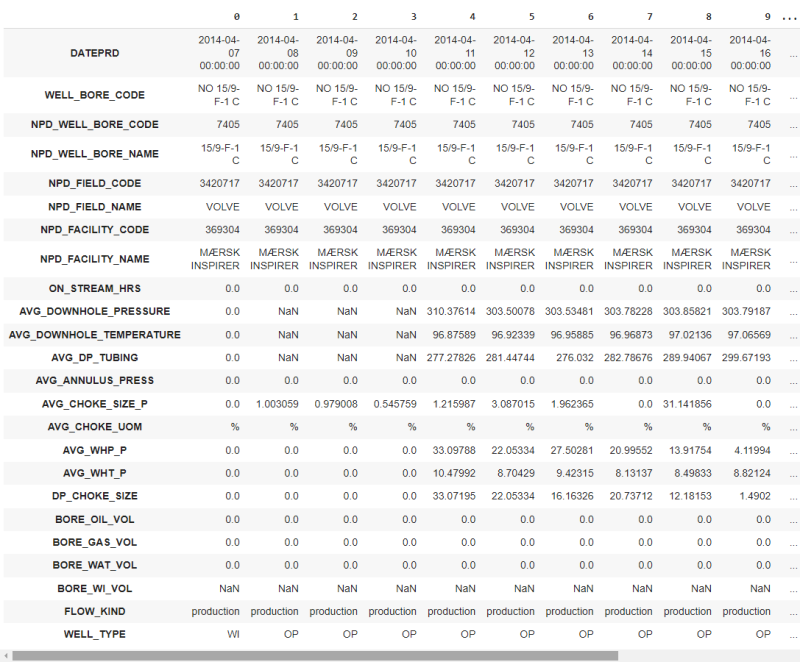
However, feature extraction from all the given data is itself a comprehensive topic, and of critical interest in this article is training the machine learning (ML) model. Therefore, I am not going to belabor all this and use only dynamic (production) data, as shown in Fig. 1 below, to train our LSTM model.
First, we do the code for oil prediction and later, this can easily be adapted for gas and water prediction with a minor modification.
To train our model, we use the data of the longest producing well (15/9-F-12). You may do a sensitivity analysis to see which input contributes the most to the output. Since it would be off-track to do a thorough analysis here. For brevity, we are using: ON_STREAM_HRS, AVG_DOWNHOLE_PRESSURE, AVG_DOWNHOLE_TEMPERATURE, AVG_DP_TUBING, AVG_ANNULUS_PRESS, AVG_CHOKE_SIZE_P, AVG_CHOKE_UOM, AVG_WHP_P, AVG_WHT_P, DP_CHOKE_SIZE, and BORE_OIL_VOL.
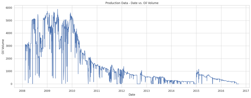
Fig. 2 below shows the plot of oil production with time (DATEPRD vs BORE_OIL_VOL) and Fig. 3 depicts our post-processing data (removing nulls, scaling the data).
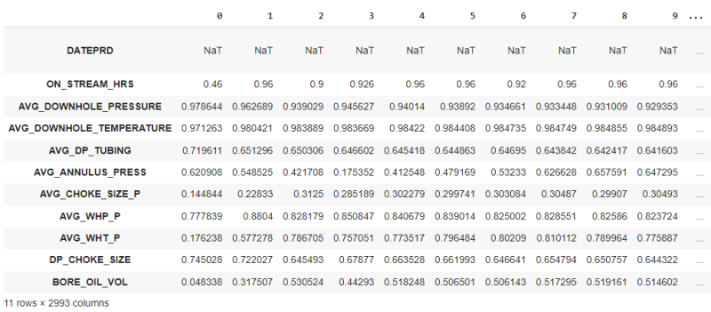
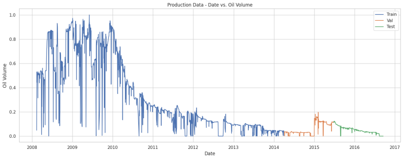
We have a total of 11 rows and 2993 columns, as indicated in the bottom left of Fig. 3. The first row is DATEPRD and we will use it only for plotting purposes. So, we have 10 rows (features). Fig. 4 below illustrates our data after splitting it into 70% training, 15% validation, and 15% test data set. Now we have:
- Number of samples in train set: 2095
- Number of samples in validation set: 449
- Number of samples in test set: 449
Here comes the most important part of our LSTM implementation:
In LSTM, we feed the data from the previous time step (previous day) and predict the target for the current time step (current day). In our case, we will feed all the features, including oil production, from the previous time step and predict the output (oil production) for the current time step. To do this, we define the “windowed_dataset” function to have features of the previous time step and the target of the current time step, as shown in the code.
We use a batch size of 32. It means that, instead of processing all our data at once, we break the data into small batches to have good speed and accuracy. Also, we use a window size (time step) of 5. It means we feed 5 days of data and predict the oil production for the 6th day.
After applying the “windowed_dataset” function to our data, we have transformed it into a 3D tensor. The shape of the input is (batch_size, window_size, features) while the shape of the output is (batch_size, window_size, target). Here,
- batch_size is 32, which means we process 32 samples at a time.
- window_size is 5, indicating that each sample spans 5-time steps or days.
- feature is 10, representing the number of input data points at each time step.
- target is 1, representing oil production for each time step.
To provide a clearer understanding, let's examine a few data for the first batch as shown below. We have 5-time steps (5 days), each consisting of 10 input data points (features) and 1 target value. Note that out of 10 input data, the last one is oil production. You can observe that the target (oil production) for day 1 becomes an input for day 2. The target for day 2 becomes an input for day 3 and this pattern continues for subsequent days. See below.
Day 1 Data:
Input data for day 1: [0.46 0.97864427 0.97126284 0.71961053 0.62090818 0.14484431 0.77783947 0.17623791 0.74502803 0.04833843]
Target (oil production) for day 2: [0.31750695]
Day 2 Data:
Input data for day 2: [0.96 0.96268884 0.98042132 0.65129648 0.54852549 0.22832986 0.8803996 0.57727789 0.72202698 0.31750695]
Target (oil production) for day 3: [0.53052377]
Day 3 Data:
Input data for day 3: [0.9 0.93902947 0.9838889 0.65030582 0.42170758 0.31249966 0.82817946 0.78670451 0.64549255 0.53052377]
Target (oil production) for day 4: [0.44293043]
Day 4 Data:
Input data for day 4: [0.926 0.94562662 0.98366927 0.64660201 0.17535249 0.2851893 0.85084674 0.75705139 0.67877023 0.44293043]
Target (oil production) for day 5: [0.51824769]
Day 5 Data:
Input data for day 5: [0.96 0.94013964 0.9842203 0.64541839 0.41254845 0.30227902 0.84067882 0.77351717 0.66352757 0.51824769]
Target (oil production) for day 6: [0.50650145]
Alright! Now it’s time to construct our LSTM model. Through experimentation with various architectures, I found that the model architecture depicted in Fig. 5 below yields the best results.
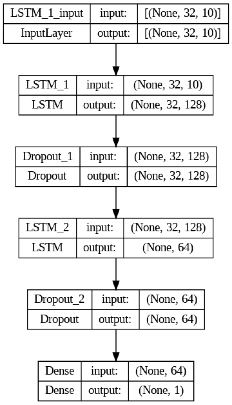
Our model comprises two LSTM layers with 128 and 64 units, respectively. Additionally, we are also using two dropout layers which is a regularization technique to prevent overfitting. In terms of optimization, we employ the Adam optimizer with a learning rate set to 0.0001 and mean squared error (mse) as the loss function. Moreover, early stopping is used to stop training early when we do not see any significant improvement on validation data set. In our setup, early stopping is activated around 400 epochs. Training and validation loss is shown in Fig. 6 below.
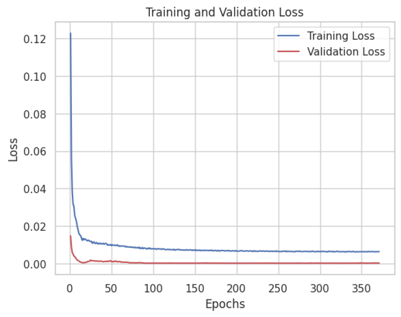
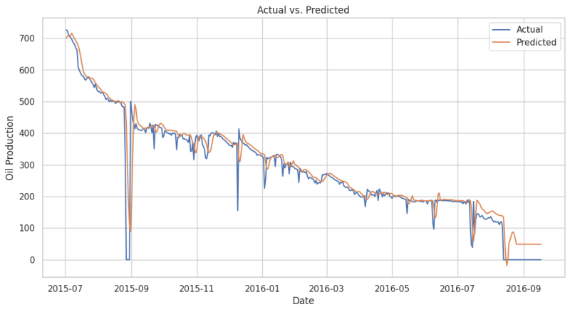
Fig. 7 presents a comparison between the actual oil production and the predictions generated by our LSTM model on the test dataset. As visible, our LSTM performs very well on that blind dataset.
If you want to train a model for gas or water, simply substitute "BORE_OIL_VOL" with "BORE_GAS_VOL" or "BORE_WAT_VOL" respectively, as directed in the code. I have trained two separate models for gas (Fig. 8) and water (Fig. 9) and the results on the blind dataset are shown below.
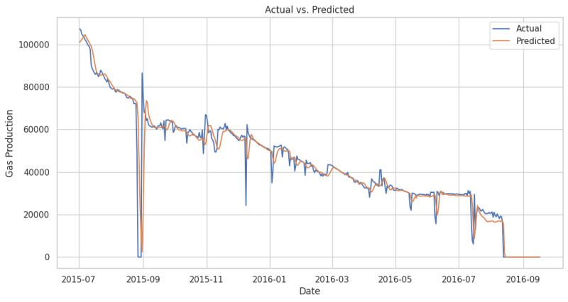
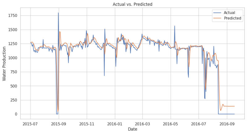
The above results indicate that the LSTM model generalizes very well for a given dataset and demonstrates strong predictive capabilities across various temporal sequences.
In the next part, we will extend our learning to a multivariate model where we will train a single model to predict three outcomes: oil, gas, and water. Until then, I encourage you to train your own model. But instead of using just one well data, use the full set of data. Try hyperparameter tunings, like more epochs, layers, etc., to have a good match. Best of luck.
