
Welcome to the concluding part of our LSTM for Production series. In Part 2, we delved into training three separate models to predict one output for each, and this is the standard practice to have separate models for the oil, gas, and water production. However, to broaden our understanding, this part will extend our learning of Part 2 to the multivariate model and train a single model to predict three outcomes: oil, gas, and water. We will use the same production data (Fig. 1) of Equinor’s Volve field. TensorFlow code for this part can be found here and I highly encourage you to follow along with it while reading this article in a separate window.
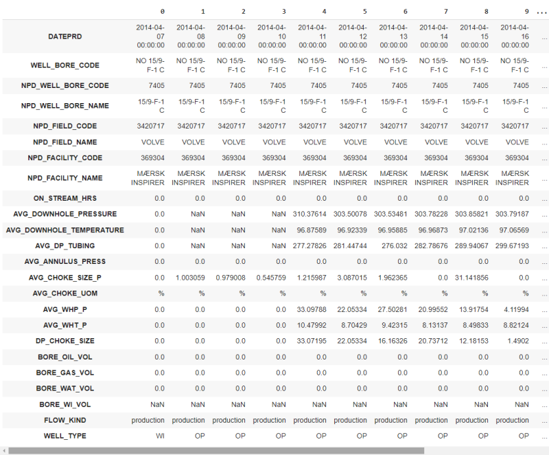
We will use the data of the longest producing well (15/9-F-12): ON_STREAM_HRS, AVG_DOWNHOLE_PRESSURE, AVG_DOWNHOLE_TEMPERATURE, AVG_DP_TUBING, AVG_ANNULUS_PRESS, AVG_CHOKE_SIZE_P, AVG_CHOKE_UOM, AVG_WHP_P, AVG_WHT_P, DP_CHOKE_SIZE, BORE_OIL_VOL, BORE_GAS_VOL, and BORE_WAT_VOL to train our model.
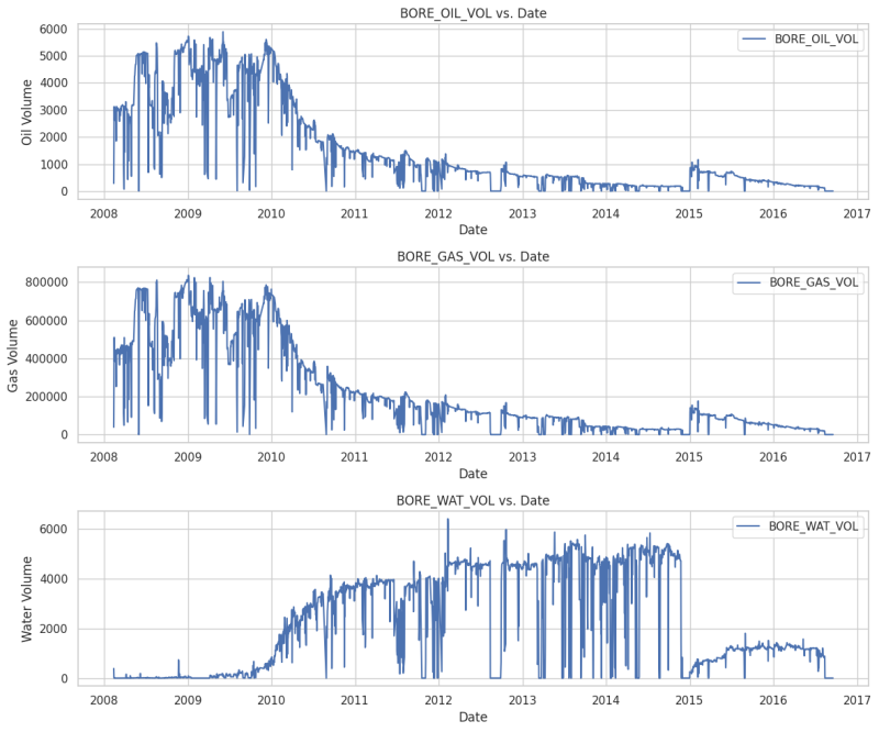
Fig. 2 shows the plot of oil, gas, and water production with time. As expected, the water volume has an opposite correlation relative to oil and gas. Additionally, Fig. 3 depicts our post-processing data (removing nulls, negative production, scaling the data).
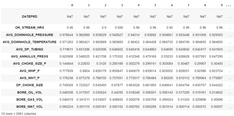
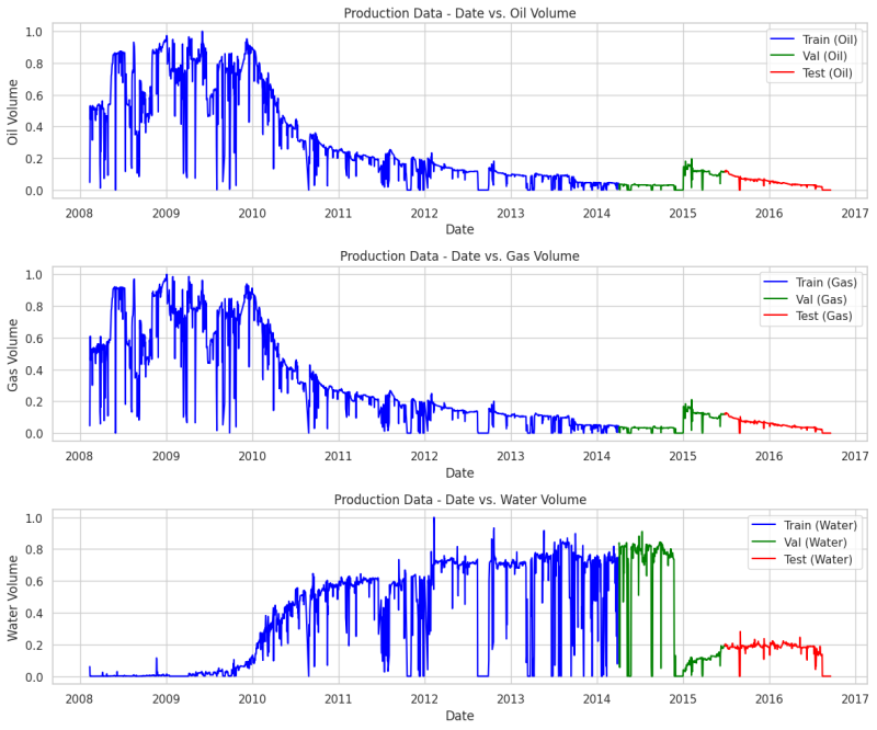
We have a total of 13 rows and 2991 columns, as indicated in the bottom left of Fig. 3. The first row is DATEPRD and we will use it only for plotting purposes. So, we have 12 rows (features). Fig. 4 illustrates our data after splitting it into 70% training, 15% validation, and 15% test data set. Now we have:
- Number of samples in train set: 2093
- Number of samples in validation set: 449
- Number of samples in test set: 449
As elaborated in the previous part, in the LSTM, we feed the data from the previous time step (previous day) and predict the target for the current time step (current day). Through experimentation, I found that, in this case, using 5-time steps (previous 5 days) as input and a single time step as output gives the best result. So, we will feed all the features (including oil, gas, and water production) of the 5 days (1st, 2nd, 3rd, 4th, and 5th days), and predict the target (oil, gas, and water production) of the 6th day. Then we will feed all the features of the (2nd, 3rd, 4th, 5th, and 6th days) and predict the target (oil, gas, and water production) of the 7th day and so forth. To do this, we define the “windowed_dataset” function to have features of the previous 5-time steps and target of the current time step, as shown in the code.
After applying the “windowed_dataset” function to our data, we have transformed our input into a 3D tensor and output into a 2D tensor. The shape of the input is (batch_size, window_size = 5, features) whereas the shape of the output is (batch_size, window_size = 1, target). Here,
- batch_size is 32, which means we process 32 samples at a time.
- window_size (for input) is 5, indicating that each sample spans 5-time steps or days.
- window_size (for output) is 1 as we are predicting the target only for one day in the future.
- feature is 12, representing the number of input data points at each time step.
- target is 3, representing oil, gas, and water production for one each time step.
To make it concrete, let's examine a few data for the first batch as shown below.
We have 5-time steps (5 days) as input, each consisting of 12 features, and output is the single time step (one day) with 3 target values. Note that out of 12 input data, the last three are oil, gas, and water production, respectively, of the previous day. You can observe that the targets (oil, gas, and water production) for the current time step becomes an input for the next time step. This pattern continues for subsequent time steps. See below.
Input Data, Five Time Step:
[[4.60000000e-01 9.78644267e-01 9.71262840e-01 7.19610527e-01 6.20908184e-01 1.44844313e-01 7.77839472e-01 1.76237915e-01 7.45028032e-01 4.83384250e-02 4.65185867e-02 6.02341404e-02]
[9.60000000e-01 9.62688840e-01 9.80421321e-01 6.51296485e-01 5.48525494e-01 2.28329865e-01 8.80399601e-01 5.77277891e-01 7.22026979e-01 3.17506950e-01 3.41211161e-01 1.11547602e-03]
[9.00000000e-01 9.39029466e-01 9.83888895e-01 6.50305816e-01 4.21707581e-01 3.12499664e-01 8.28179460e-01 7.86704514e-01 6.45492548e-01 5.30523767e-01 6.10007499e-01 1.81479969e-04]
[9.26000000e-01 9.45626620e-01 9.83669275e-01 6.46602008e-01 1.75352493e-01 2.85189302e-01 8.50846736e-01 7.57051390e-01 6.78770230e-01 4.42930431e-01 4.58654585e-01 1.51754802e-04]
[9.60000000e-01 9.40139637e-01 9.84220296e-01 6.45418394e-01 4.12548449e-01 3.02279023e-01 8.40678816e-01 7.73517171e-01 6.63527573e-01 5.18247692e-01 5.00578165e-01 7.65031939e-04]]
Output Data, One Time Step:
[5.06501446e-01 5.05708662e-01 2.89429261e-04]
Next Input Data, Five Time Step:
[[9.60000000e-01 9.62688840e-01 9.80421321e-01 6.51296485e-01 5.48525494e-01 2.28329865e-01 8.80399601e-01 5.77277891e-01 7.22026979e-01 3.17506950e-01 3.41211161e-01 1.11547602e-03]
[9.00000000e-01 9.39029466e-01 9.83888895e-01 6.50305816e-01 4.21707581e-01 3.12499664e-01 8.28179460e-01 7.86704514e-01 6.45492548e-01 5.30523767e-01 6.10007499e-01 1.81479969e-04]
[9.26000000e-01 9.45626620e-01 9.83669275e-01 6.46602008e-01 1.75352493e-01 2.85189302e-01 8.50846736e-01 7.57051390e-01 6.78770230e-01 4.42930431e-01 4.58654585e-01 1.51754802e-04]
[9.60000000e-01 9.40139637e-01 9.84220296e-01 6.45418394e-01 4.12548449e-01 3.02279023e-01 8.40678816e-01 7.73517171e-01 6.63527573e-01 5.18247692e-01 5.00578165e-01 7.65031939e-04]
[9.60000000e-01 9.38920170e-01 9.84408049e-01 6.44863216e-01 4.79168806e-01 2.99740521e-01 8.39014000e-01 7.96483690e-01 6.61992601e-01 5.06501446e-01 5.05708662e-01 2.89429261e-04]]
Output Data, One Time Step:
[0.50614313 0.49502421 0.00101378]
Next Input Data, Five Time Step:
[[9.00000000e-01 9.39029466e-01 9.83888895e-01 6.50305816e-01 4.21707581e-01 3.12499664e-01 8.28179460e-01 7.86704514e-01 6.45492548e-01 5.30523767e-01 6.10007499e-01 1.81479969e-04]
[9.26000000e-01 9.45626620e-01 9.83669275e-01 6.46602008e-01 1.75352493e-01 2.85189302e-01 8.50846736e-01 7.57051390e-01 6.78770230e-01 4.42930431e-01 4.58654585e-01 1.51754802e-04]
[9.60000000e-01 9.40139637e-01 9.84220296e-01 6.45418394e-01 4.12548449e-01 3.02279023e-01 8.40678816e-01 7.73517171e-01 6.63527573e-01 5.18247692e-01 5.00578165e-01 7.65031939e-04]
[9.60000000e-01 9.38920170e-01 9.84408049e-01 6.44863216e-01 4.79168806e-01 2.99740521e-01 8.39014000e-01 7.96483690e-01 6.61992601e-01 5.06501446e-01 5.05708662e-01 2.89429261e-04]
[9.20000000e-01 9.34661316e-01 9.84735168e-01 6.46949520e-01 5.32329634e-01 3.03084030e-01 8.25001569e-01 8.02090048e-01 6.46641243e-01 5.06143132e-01 4.95024213e-01 1.01378466e-03]]
Output Data, One Time Step:
[5.17295018e-01 5.13430126e-01 1.14207222e-04]
Great! Now let's proceed with the construction of our LSTM model. I opted to use the same architecture (Fig. 5) we used in Part 2. Fig. 6 shows its results on a blind dataset.
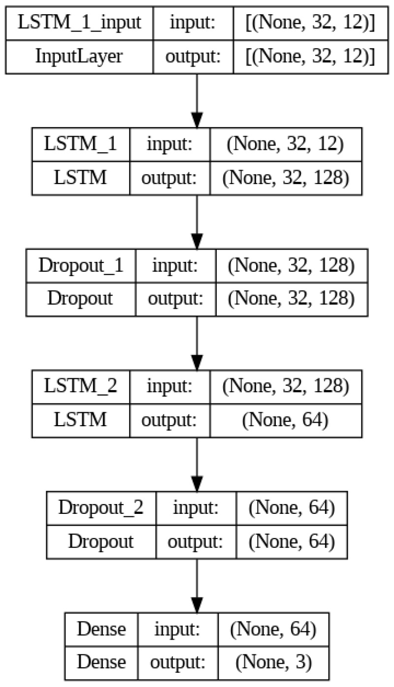
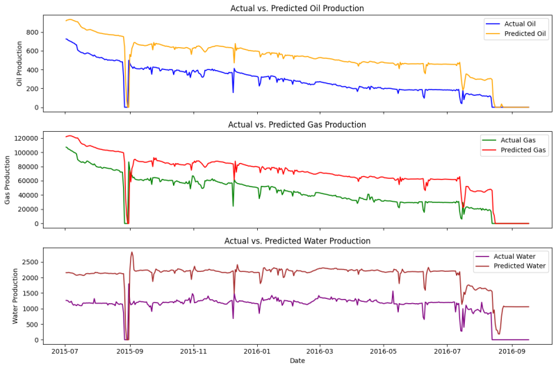
As evident in Fig. 6, the LSTM performs very poorly when it comes to predicting three different outputs. The main reason, I hypothesize, is water production which has a contrasting pattern compared to the other two outputs (oil and gas). Hence, our model has difficulty learning different trends. I have experimented with various hyperparameters and a custom loss function in an attempt to have a good fit for all three. Unfortunately, they were all in vain.
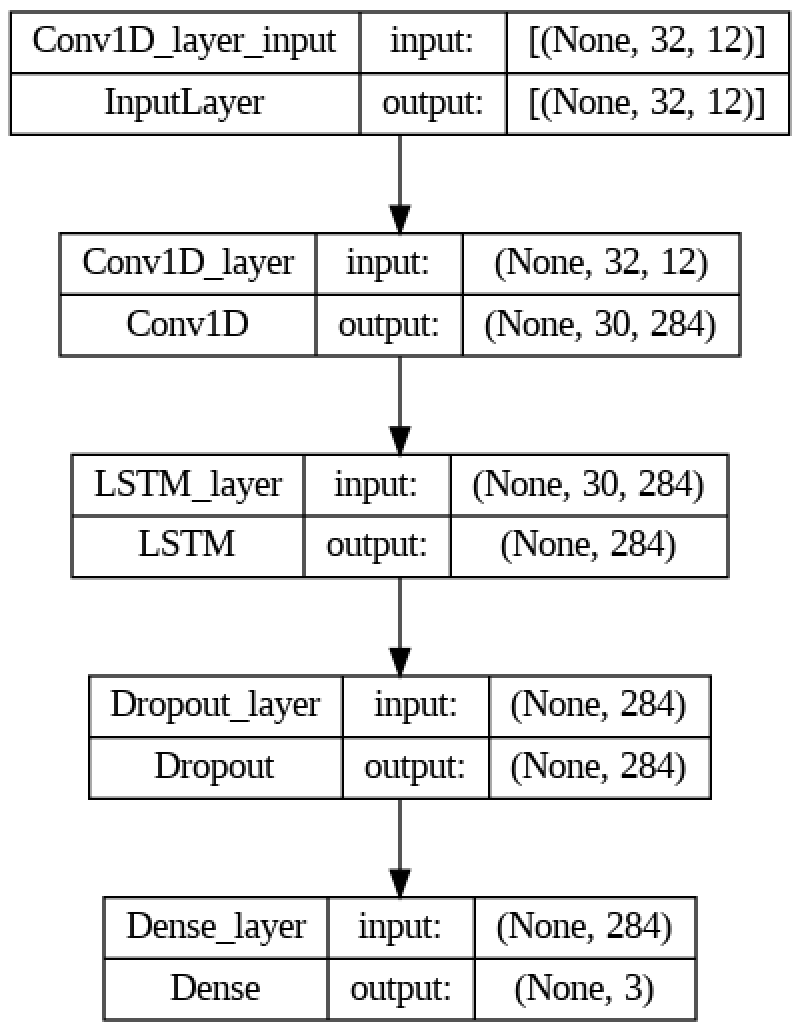
However, a combination of LSTM with convolutional neural network (CNN) yielded the most favorable results. This combined model is named the Long- and Short-Term Time-Series Network (LSTNet). The convnet looks for patterns anywhere in the input time series. It transforms the long input sequence into much shorter, down sampled sequences comprising higher-level features. This sequence of extracted features then becomes the input to the LSTM component of the network.
Our LSTNet model architecture, as depicted in Fig. 7, is: one Conv1D layer with 284 filters and a kernel size of 3, followed by an LSTM layer with 284 units and a relu activation function, then a dropout layer with a rate of 0.5, and finally, one dense layer with 3 units and a sigmoid activation function. The Adam optimizer with a learning rate of 0.0001 and mean squared logarithmic error as the loss function are being used. Similar to the previous part, early stopping is used to stop training early when we do not see any significant improvement on a validation data set. In this setup, early stopping is triggered around 300 epochs. The performance of the model on a blind dataset is illustrated in Fig. 8.
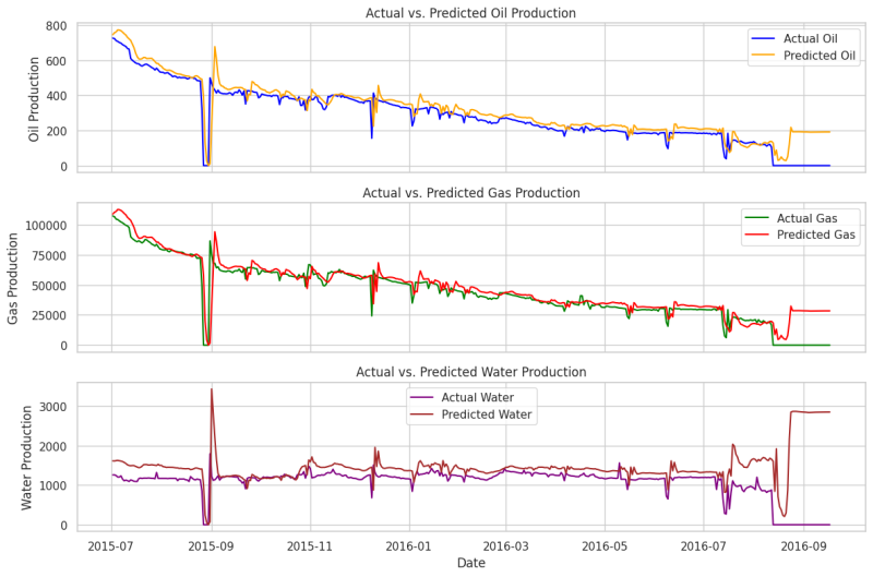
This result (Fig. 8) is quite good, though not perfect for water, especially at the tail. You may try further hyperparameters tunning to have an excellent fit for water as well.
Until now, we used only production data to forecast the future production of a well, but at the end of the day, this is the empirical decline curve analysis (DCA). Reservoir characteristics, completion design, or production constraints do not play any role in the DCA. Moreover, DCA completely ignores the water or gas injection rates.
Therefore, it would be unwise to employ machine learning to tackle DCA. In the parlance of full field modeling, it is very important to include the spatial data (static), along with temporal data (dynamic) in the model. For instance, porosity, permeability, thickness, perforation, and offset wells data, just to name a few. My future articles will be on this topic (preparing spatio-temporal datasets for machine learning).
Thank you for your time and stay tuned for more freshly brewed content!
