
By Yuxing Ben, SPE, Occidental; Naveen Krishnaraj, SPE, University of Houston; Sarath Pavan Ketineni, SPE, Chevron Corporation, and Pushpesh Sharma, SPE, Aspen Technology
Introduction
Shear sonic logs can be used to calculate the rock mechanics properties of a formation, which is useful for geomechanics studies in the development of oil and gas fields. Shear sonic logs, however, are not often measured compared with other well logs. Empirical equations, such as Greenberg-Castagna relations, can be used to estimate shear sonic logs, but they only work for brine-saturated rocks (paper SPE 198764). Some efforts have been made to use machine learning to generate synthetic logs, and these obtained some positive results. The studies in the literature typically use the data from just a couple of wells, which makes scaling up the machine-learning solutions to other wells difficult.
The SPE Gulf of Coast Section’s (GCS) Data Analytics Study Group is grateful to TGS, which provided shear sonic logs from 234 wells. Although the well names were not available, machine-learning practitioners who took part in the SPE-GCS Data Analytics Study Group’s Machine Learning Challenge 2021 still could use this relatively large data set to learn through applying different machine-learning work flows to it. There were several obstacles to organizing this event, but there was a broad interest from technical professionals across the globe in this local section event; SPE had not held such a competition before. The quality of the machine-learning solutions submitted for this competition was very high. Therefore, we would like to share our experience in organizing such an event and the technical merits of doing so. We hope that other SPE sections can hold similar competitions in the future to encourage innovation among their technical communities.
How Was the Competition Organized?
This competition started on 15 January 2021, when TGS provided the data from 234 wells. The data included various well logs such as gamma ray, porosity, resistivity, and compressional slowness. The data were shared via Dropbox folders. We organized the following three webinar workshops for the people who were new to machine learning:
- Data Engineering, presented by Babak Akbari
- Data Modeling, presented by Sunil Garg
- Hyperparameters Tuning, presented by Shivam Agarwal and Manisha Bhardwaj
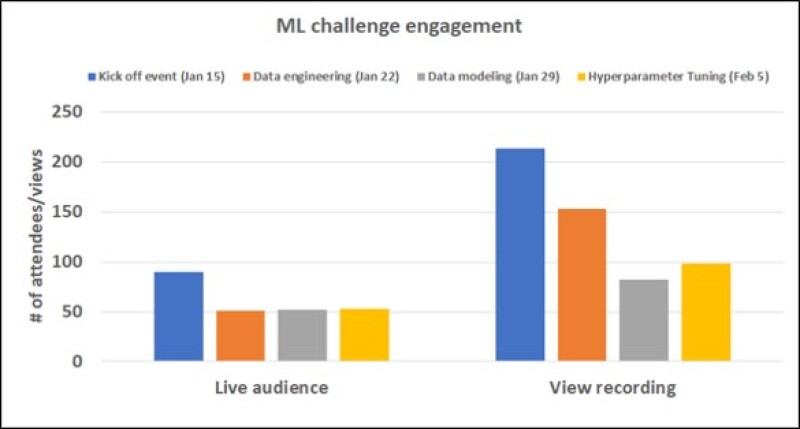
Fig. 1 summarizes the number of people who participated in these webinars.
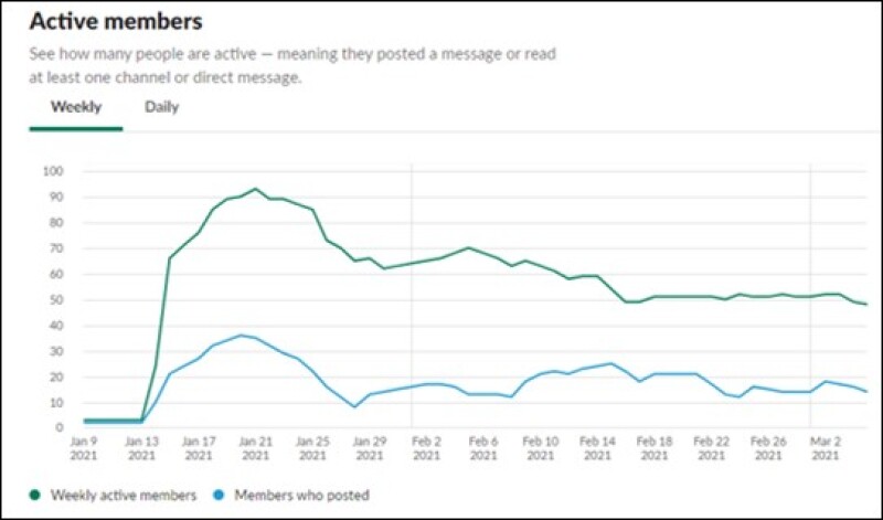
The team communicated through a Slack channel. Fig. 2 records the Slack channel activities by date. Nineteen teams joined the competition and submitted final results. These teams included early-career petroleum professionals as well as graduate and undergraduate students. The teams were from the US, Canada, India, and Indonesia. The data for the first round of test wells for leaderboard purposes were sent out on 1 February 2021. The final 20 wells were sent out for testing on 14 February. The metrics were determined by root mean square error (RMSE).
The leaderboard was created using a script internally developed by the team. The top 10 teams submitted a 5-minute video presentation and their code. Three judges (Yuxing Ben, Manisha Agarwal, and Douglas Dohmeyer) looked at the solutions from the top 10 teams on the leaderboard. Awards were presented to the top three winners, and two innovation awards were given based on the teams’ solutions. The codes and presentations of the teams are available in this Github repository.
What Have We Learned From Organizing the Event?
This is the first time that SPE organized such a machine-learning competition. All the organizers were volunteers, each either being a full-time student or having a full-time job. Not only did they lack experience planning competitions but they also lacked the time to support the event exclusively. The following lessons were learned:
- Platform—The organizers reached out to some providers who could host a machine-learning competition online, but that did not work out, so a manual process was used to create and manage the leaderboard. This demanded more work than expected. The organizers would rather engage platforms to hold the competition online in the future. This would allow for more frequent leaderboard feedback to participants.
- Code Submission—Two requirements were set for the code: that it be easy to understand and easy to reproduce. Some groups submitted Python files, while others submitted Jupyter Notebooks, which were easier to understand than the Python files. Very few groups shared the system and package requirements to run the code. The reviewers and judges spent hours reading and reproducing the code. Organizing a seminar by a software-development professional to guide the participants on generating reproducible and readable codes may be a good idea for future events.
- Duration of the Competition—Participants were given 7 weeks to submit their results. This seemed to be too short based on the feedback from some participants. Some of the submitted presentations missed a lot of good efforts reflected in the code. If the participants were given more time, the quality of the presentations and the code may have been even better.
- Data Sharing—Organizers need to ensure the data are sufficient and good enough for a competition. We are grateful that TGS provided the data for this competition. These data had different formats and required a lot of data preprocessing to train a machine-learning model, which was a challenge for the participants. We hope more companies will share their data with the SPE community to help the industry find better data solutions.
Machine Learning Solutions From the Teams
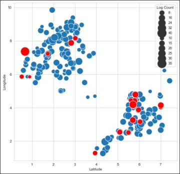
Overview of the Raw Data and Test Data. The raw data were from 234 wells located in two relatively separate geoclusters. The data included depth, longitude, latitude, shear slowness (DTSM), compressional slowness (DTCO), density log, gamma ray, photoelectric factor, neutron porosity (NPHI), resistivity, and caliper logs. Only depth, latitude, longitude, and DTSM data were available for every well. Most of the wells had multiple logs with the same units because they were obtained from different sources.
Fig. 3 shows the location of each well, forming two geoclusters. The blue solid circles represent the wells in the training data set, while the red solid circles represent the test wells, which could belong to either one of the geoclusters. The sizes of the circles represent the number of available logs, which varied considerable for the different wells. These challenges must be sorted out before building a machine-learning model. Sri Poludasu, who ranked No. 1, did a wonderful job on data exploratory analysis in his submitted Jupyter Notebook. Please refer to his solution on Github for more information.
Feature Engineering. For many published works on machine learning in the petroleum industry, the authors will first perform feature engineering, then will spend a lot of effort on selecting the best models based on different machine-learning algorithms and tuning hyperparameters. Unfortunately, the data used in such papers are not available to share, so it is hard to tell why one machine learning approach is better than the other. The power of having different teams work on the same data set is that each team will come up with its own feature engineering strategy. What matters is not only the machine learning model but also the feature engineering methodology.
One interesting observation is that the top five teams all considered the location of the wells, while the teams that placed sixth through tenth did not use the location as a feature. The No. 8 team creatively explored many data-science techniques, such as using moving windows and a recurrent neural network, but their accuracy was not as high as the top seven teams. This suggests the importance of location for accurate well log predictions.
The No. 1 team created a compound feature by averaging the repeatable measurements for the same type of logs. The rest of the teams usually eliminated duplicated logs with the same mnemonics. We suspect that the created compound feature enabled the model to use more available data, reducing the errors for some of the input variables and improving the model’s accuracy.
Outlier Remover. A lot of teams used domain knowledge to remove the outliers. For example, Team No. 2 removed the bad holes from the data, Team No. 1 removed some correlation logs, and Team No. 5 applied a median filter to remove spike noise.
Missing Values. Every type of well log was not available for every well. How the teams filled in missing values was typically not shown in their final presentation slides. Based on the code review, the No. 1 team and the No. 8 team filled in missing values using the IterativeImputer class in the scikit-learn package of Python. This class models each feature with missing values as a function of other features and uses that estimate for imputation. It does so in an iterated round-robin fashion: At each step, a feature column is designated as Output y and the other feature columns are treated as Inputs X. A regressor is fit on (X, y) for known y. Then, the regressor is used to predict the missing values of y. This is iteratively done for each feature and then is repeated for maximum iteration imputation rounds. The No. 2 team used the “ffill” or “bfill” method in pandas.DataFrame to fill in missing values, where “ffill” means “forward fill” and “bfill” means “backward fill.” The No. 4 team developed its own machine-learning regressors for different features to fill in the missing values. The typical inputs for the regressors are the known values, the depth, and the locations of the wells.
Training Data Set Selection. A lot of values were missing from the training data set as well as from the test data set. The column names in the training data set are not the exact ones used in the test wells, so the teams had to design a work flow to accommodate this. The No. 1 team did a thorough column name analysis and used the whole data set after filling in the missing values. The No. 2 team picked the wells closer to the test wells and used them as the training data set. It was hard to tell which strategy was better, but both teams ranked at the top.
Models. Different teams used different machine learning models, such as Light GBM, XGBoost, and neural networks. The No. 1 team used random forest and XGBoost, and selected XGBoost for result submission. The No. 2 team used a neural network with a rolling window. The No. 3 team explored XGBoost, random forest, and an artificial neural network and chose XGB as their final model. Interestingly, the No. 4 team used AutoRegressor in jcopml.automl (a machine learning package in Python), which allowed them to try different machine-learning models including random forest, XGB, KNeighbors, ElasticNet, and support vector regression. The automl (automatic machine learning) ranked random forest the best algorithm for the selected features. The No. 8 team used several machine-learning algorithms, including recurrent neural network, but they neglected the locations of the wells in the feature selection such that they could not achieve better RMSE than the top seven teams. Therefore, feature engineering proved to be as important as the machine learning model.
Results
Table 1 is the final leaderboard. Column 2 shows the RMSE achieved by the different teams. The smaller the RMSE is, the better the machine learning algorithm is. As shown, the results from the top teams are very close, but the result of team No. 1 is almost 9% better than that of the No. 5 team. We think that the compound feature created by the No. 1 team and the use of IterativeImputer class in Python helped the No. 1 team win.
| Team Name | RMSE |
| Sri Poludasu | 22.90572367 |
| Shruggie | 23.74729592 |
| Team Geoexpert | 24.3914156 |
| Samsan Tech | 24.71052856 |
| The Viet TU | 24.91721614 |
| Shear Waves | 25.35753255 |
| Doalbu | 25.39167717 |
| The Panda | 25.72346706 |
| Diggers | 26.53351134 |
| Osiris of AI | 28.0394755 |
| Ganesha20 | 28.39456464 |
| Payel Ghosh | 28.49074566 |
| Data Driller | 29.14519749 |
| Space Troopers | 30.30963618 |
| The ReSteam | 30.72574474 |
| Jeremy Zhao | 30.87261698 |
| Thunderbird | 31.3251757 |
| Virtual Kwell LoggerS | 33.89327656 |
| AIgators | 34.72068233 |
| Table 1—Leaderboard. | |
Discussion
The technical summary is based on the authors’ understanding of the presentations from the top 10 teams and the code submitted by the teams; it may not fully reflect the full efforts of the different teams. What encourages us is the novelty of the different approaches that the teams had taken. A good machine-learning application should leverage domain knowledge, have a good feature engineering strategy, and choose the appropriate machine-learning model. We believe that data science will be used increasingly in the oil and gas industry to improve work efficiency and reduce costs, which is why we are sharing the lessons learned during this competitive SPE event.
Acknowledgments
We want to acknowledge the Machine Learning Challenge organizing team: Pushpesh Sharma, Babak Akbari, Suresh Dande, Sunil Garg, Diego Molinari, Manisha Bhardwaj, and Shivam Agarwal. We would like to convey our heartiest gratitude to Alejandro Valenciano and CenYen Ong of TGS for their support during the data sponsorship process, and Erica Coenen of Reveal Energy Services for her support with event sponsorship. We would also like to thank Jeanne Perdue from Occidental for reviewing the manuscript.
This information presented here is based on the authors’ affiliation with the SPE Gulf Coast Section Data Analytics Study Group and does not represent their companies’ interests or viewpoints.