Production forecasting is a crucial task in reservoir management and reservoir development decisions. Because of the limitations of uncertain geological conditions, production history, data quality, and uncertain operational factors, however, it is difficult to accurately predict the well production over time. This article presents a deep-learning approach, the long short-term memory network, for adaptive hydrocarbon production forecasting. The method takes historical operational and production information as input sequences to predict oil production as a function of operational plans.
Volve Data Set
Equinor’s Volve data set is a publicly available subsurface data set. Well 15/9-F-12 from the Volve data set is used in this study to demonstrate the effectiveness of the adaptive production forecasting methodology. The data set is named after the Volve oil field, which was discovered in 1993 and produced oil from 2008 to 2016 in the North Sea, offshore Norway. For production forecasting, multiple features were considered that include onstream hours, average bottomhole pressure and temperature, wellhead pressure, choke size, as well as daily hydrocarbon production.
Long Short-Term Memory (LSTM) Network
The proposed LSTM neural network model for production forecasting accounts for well productivity and operational variabilities. It is designed for time-dependent data and can retain long-term dependence while maintaining accuracy over short time scales. LSTM networks are ideal for processing sequential data because of their unique memory cell and gating mechanism, which selectively stores and retrieves information over time. This makes them suitable for handling forecasting problems that require consideration of past and present inputs and outputs.
LSTM Hyperparameters. Hyperparameter tuning is necessary for improving the performance of production forecasting. Hyperparameter tuning offers advantages such as performance enhancement, generalization, and computational resource savings. It is important to note that hyperparameter tuning can be a time-consuming process. It is important to avoid overfitting the model to the validation set, which can lead to poor performance on unseen data. Using cross-validation techniques evaluating the final model on a separate test set, therefore, is important. The choice of hyperparameters governs the final structure of the LSTM network best suited for the production forecasting for the Volve data set (Fig. 1).
The following are a few of the more important hyperparameters of LSTM and their roles:
- Number of LSTM units—This hyperparameter determines the number of memory cells (or LSTM units) in each LSTM layer. A higher number of LSTM units allows the model to remember more information but also increases the computational cost and the risk of overfitting. For the best model accuracy, we used 128 and 64 units in our model.
- Number of LSTM layers—This hyperparameter determines the depth of the LSTM network. A deeper network allows the model to capture more complex patterns in the input sequence but also increases the risk of overfitting. In our model, two LSTM layers were enough to build the neural network.
- Learning rate—This hyperparameter controls the step size of the gradient descent algorithm during training. A higher learning rate allows the model to learn faster but can also cause the model to overshoot the optimal solution and converge to a suboptimal solution. A lower learning rate, in our case 0.0001, allows the model to converge more slowly but also prevents it from escaping local minima.
- Dropout rate—Dropout is a regularization technique that helps prevent overfitting by forcing the model to learn more robust features. A higher dropout rate can increase the model’s ability to generalize but can also decrease the model’s capacity to learn complex patterns. For the best model performance, we proposed two dropout layers with a rate of 0.5 for each to properly remove a certain fraction of LSTM units during each iteration.
- Batch size—This hyperparameter determines the number of samples that is processed in each training batch. A larger batch size can speed up the training process and improve model stability, but it also increases memory usage and the risk of overfitting. Given this, we chose a batch size of 32.
- Activation function—This hyperparameter introduces nonlinearity into the model. Activation function is applied to the LSTM units. In our case, the ReLU and Linear activation functions are used. Choosing the best activation function can help the model learn more accurate representations of the input sequence.
- Early stopping—By using early stopping, the model can be trained in less time, reducing the risk of overfitting and improving the model’s generalization performance. Additionally, early stopping can save time and resources that would otherwise be wasted on training an overfitted model.

Time-Series Nested Cross Validation. To train and tune the LSTM network on time-dependent data, time-series nested cross-validation is used. It evaluates the model’s performance and selects hyperparameters while accounting for the temporal ordering of the data. The data is split into multiple folds, with each fold consisting of a contiguous block of time (Fig. 2). The folds are divided into an outer and inner loop. In the outer loop, a sliding window approach is used to split the data into training and testing sets. In the inner loop, each training set is further split into a training and validation set and multiple models are trained with different hyperparameters. The best-performing hyperparameters are selected based on the validation set. Our work uses fivefold time-series nested cross validation, with the average performance of the five folds measured using the mean squared logarithmic error (MSLE). This cross-validation method searches for hyperparameters that best learn from various chronological sequences of the time-dependent data and evaluates the model’s performance on the remaining chronological sequence.

Loss Function. The loss function represents the function that evaluates the difference between the prediction of the LSTM network model under training and the actual output used for the training. In our LSTM model, the MSLE is used as a proxy for the loss function. The MSLE is defined as the mean of the squared variances between the expected and actual values’ natural logarithms.
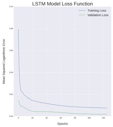
The loss is computed for each iteration of the LSTM model in order to determine the current model’s performance. In this case, the model will be stopped early if the validation loss increases because, when the validation loss starts increasing after several training sessions, that indicates the model is overfitting for some pattern in the training data. Fig. 3 shows the drop in loss curves for training and validation stages as the LSTM network is trained over 120 epochs. Early stopping is activated around 120 epochs.
Adaptive Production Forecasting Using the LSTM Network
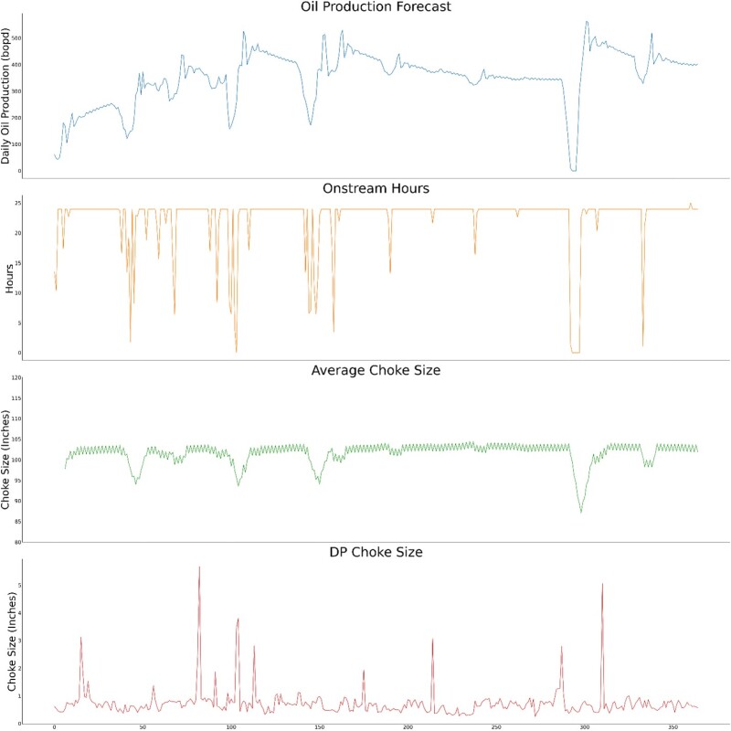
Input and Output Sequences. The overall forecasting work flow, as depicted in Fig. 4, uses a sequence-to-sequence strategy with 10 historical operational and production sequences, in addition to three future operational sequences, to predict one future production sequence. We performed extensive hyperparameter tuning for the LSTM model to find that using 5 days of 10 historical production and operational sequences along with 5 days of three future operational sequence are best suited to predict 5 days of oil production sequence. These three operational parameters are onstream hours, average choke size, and differential pressure (DP) choke size. The adaptive production forecasting uses both historical information along with operational plans to predict oil production.
Specifically, our forecasting work flow uses 10 operational and production parameters for time indices n-5 through n-1 to represent the previous 5 days. These 10 historical sequences are used as input sequences for the LSTM network. Additionally, the values of three specific operational parameters for time indices n through n+4 are used as future feature sequences. Together, these 13 sequences serve as the input features for the LSTM model, which predicts one oil production sequence for the following 5 days (time indices n through n+4). Fig. 4 elaborates the 13 input sequences and one output sequence.

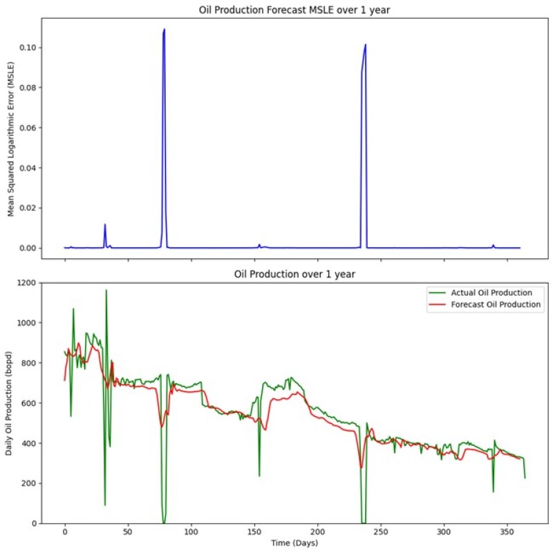
Model Evaluation. After the training and tuning, we perform the forecasting for a period of 1 year, 5 days at a time, on the test data that was kept separate. To assess the accuracy of our forecasting model, we used the MSLE metric when evaluating the model’s performance on the testing set. Errors in forecasting are low except around 70 days and 230 days (shown at the top in Fig. 5). LSTM performs very well during normal scenarios, except at the two instances when there were sudden shutdowns. However, the LSTM model can handle changes in the production that are not very large (e.g., large shutdowns) very well. In Fig. 5, the actual oil production profile of the test data is shown in green and the forecasted production profile is shown in red. The blue curve at the top in Fig. 5 shows the forecasting error in terms of MSLE.
Model Deployment for Adaptive Production Forecasting. Deployment happens after the completion of the training/testing stage. To demonstrate the deployment of the adaptive production forecasting method, we changed only three operational parameters—onstream hours, average choke size, and DP choke size—as shown in Fig. 5, which represent the future operational sequences used as input to LSTM. The remaining input sequence were kept constant. Fig. 6 shows the forecast of the oil production for 1 year, being predicted 5 days at a time. In the deployment stage, the performance of the model cannot be evaluated because of the lack of measured data, which is available only for training and testing stages. Fig. 6 confirms that the adaptive production forecasting methodology can learn from the historical data to predict the oil production that is sensitive to changes in onstream hours, average choke size, and DP choke size. The adaptive production forecasting methodology can successfully learn from the training data for deployment over a period of 1 year.