

Drilling long horizontal wellbores and completing wells with multistage fracturing are common practices in shale-play development. One of the keys to enhancing production of these ultratight reservoirs is the creation of a complex fracture system with very high surface area. Results of the current study show that post-treatment production data exhibit distinct features associated with various fracture systems and should be able to aid in describing the complex fracture system. The primary objective of this work was to find correlations between early-time production signatures and the fracture network.
Introduction
Hydraulic fracturing has long been an effective technique for stimulating low-permeability reservoirs. To simplify fracture modeling, biwing single-plane fracture geometry was often assumed from prefracture design through post-fracturing evaluation. However, fractures in the real world have been documented to be much more complex. Especially for economic shale plays, hydraulic-fracture interaction with natural fractures may result in complex fracture-network development. The biwing-fracture parameters—length, height, width, and conductivity—are not sufficiently detailed to describe complex fractures. Instead, another set of parameters—fracture density, unpropped- and propped-fracture conductivity, and stimulated-reservoir volume (SRV)—may be more-appropriate parameters to consider in both fracture design and production modeling.
After fracturing treatments, characterization of created fracture profiles helps engineers to understand the reservoir better and thereby to optimize subsequent well completions. Various fracture-diagnostic technologies were developed to describe the fracture parameters involved: orientation, length, height, width, and conductivity. These fracture-diagnostic techniques have been applied mainly to estimate biwing-fracture geometry. When applied to shale-gas wells, some of them fail to provide helpful information because of the complexity of the created fracture network.
Microseismic mapping is a technique that is widely accepted to characterize complex fracture networks. However, it is difficult to estimate the effectiveness of stimulation treatments directly from microseismic mapping because the location of proppant and the distribution of conductivity in the fracture network cannot be determined from microseismic data.
Direct fracture-diagnostic methods and production-analysis techniques are beyond the scope of this work. But, informed by the ideas underlying those techniques, this paper attempts to identify possible correlations between early-time production signatures and complex-fracture-system parameters.
Simulation Models
Production-simulation models for multistage fracturing of horizontal wells also become very complex when trying to capture merely the major physics involved. Because this work discusses only early-production signatures of shale-gas wells, desorption is not taken into account here. For most shale plays, desorption of gas starts to contribute significantly only after the reservoir pressure drops to a relatively low level. The simulation model used in this study considers a horizontal well with eight stages of transverse hydraulic fractures, each of which is associated with an induced SRV. In the middle of each SRV, a propped fracture (referred to as the “primary fracture” in the rest of this paper) is represented by a plane of simulation cells with high conductivity. Logarithmically spaced and locally refined gridblocks are used to correctly represent fluid flow perpendicular to the primary-fracture faces. Within each SRV, a uniformly distributed network of fractures, which are denoted as “secondary fractures,” is assumed. The first 3 years of production are simulated for each case.
A dual-porosity, dual-permeability model is adopted in this study to represent the SRV. It represents the fractured reservoir with a matrix domain and a fracture domain. The fracture network consists of primary and secondary fractures. The primary fracture is connected to the wellbore and is oriented perpendicularly to the direction of the horizontal wellbore. It is assumed in this model that the matrix domain and the secondary fractures have no direct communication with the wellbore. The flow from the matrix to nearby fractures is assumed to be quasisteady state. The capacity of fluid interaction between the matrix and the fracture network is determined by the fracture spacing and matrix permeability.
After fracturing treatment, the created fractures are filled with fracturing fluid. Depending on reservoir and fracture properties, it can take days to months to clean up those fractures. During this flowback period, the single-phase flow assumption does not hold true. In this study, the model is initialized in a way that can address multiphase flow during the early production stage. The matrix domain is initialized with reservoir pressure and fluid saturations, while the fracture domain is initialized with 100% water saturation.
Models are set up with various combinations of secondary-fracture distribution and conductivity, primary-fracture conductivity, and different sizes of SRV. Different simulation cases were performed with network fracture spacing varying from 25 to 100 ft, secondary-fracture conductivity from 1 to 7 md-ft, primary-fracture conductivity from 100 to 1,000 md-ft, and three sizes of SRV.
Results and Analysis
Production signatures at different productivity periods of the well’s life are dominated by different fracture parameters. If the peak production time is set as the reference point, secondary-fracture-density differences can be indicated by the production-decline rate after peak production; secondary- and primary-fracture conductivities are more reflected by the gas-production signature before the peak; and different SRV sizes show the same signatures before the peak and the same decline rate but different absolute gas rates after the peak.
Production signatures can be interpreted better by using diagnostic plots. Four types of plots are selected to identify production signatures that could be used to characterize the hydraulically generated fracture parameters. Of these plots, reciprocal of gas-flow rate vs. gas-material-balance time and the reciprocal of gas-rate derivative vs. time are provided in this summary. Each of these analysis plots consists of four groups to show the effect of secondary-fracture spacing, secondary-fracture conductivity, primary-fracture conductivity, and SRV, respectively.
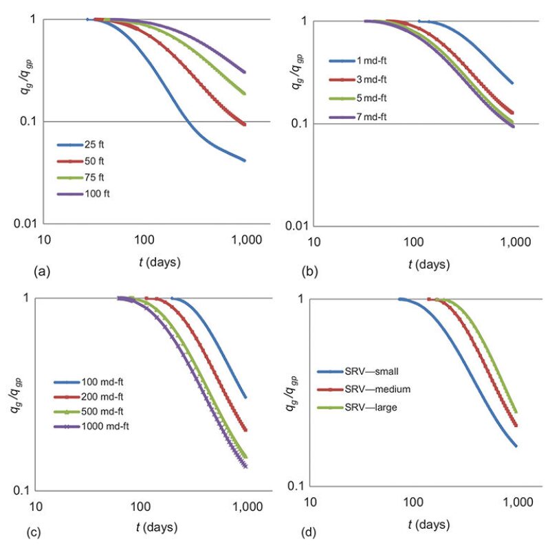
Reciprocal of Gas-Flow Rate vs. Gas-Material-Balance Time. Log-log plots of reciprocal of gas flow rate vs. gas-material-balance time have been applied to estimate gas reserves of dry-gas reservoirs. To achieve this end, it was assumed that single-phase flow and boundary-dominated flow had been developed. Study scenarios in this paper do not meet those requirements. However, grouping together this plot for different simulation cases still provides valuable information in terms of fracture characterization. Fig. 1 above plots the reciprocal of gas flow rate vs. gas-material-balance time in log-log coordinates. All four groups of curves share the same general trend. With increasing gas-material-balance time, the reciprocal of gas-flow rate decreases first, which represents the fracture-cleanup period. After reaching a minimum value, which represents the peak rate of production, each curve starts to increase with gas-material-balance time.
Fig. 1a illustrates the plots for four simulation models with different secondary-fracture spacing. Before reaching peak production rate, gas-flow rates for all the four cases increase with approximately the same slope. After the peak, the four curves demonstrate different slopes. The smaller the secondary-fracture spacing, the steeper the curve. It can be interpreted that more-intensively-spaced complex fracture networks deplete shale-gas reservoirs more quickly. What is also worth pointing out is that all four cases reach maximum production rate at approximately the same gas-material-balance time, although the absolute peak values are different. Models plotted in Fig. 1b have varying secondary-fracture conductivity. The most important observation from this plot is that different gas-material-balance times are required for the four cases with varying network fracture conductivity to reach maximum production rate, which suggests that higher network fracture conductivity helps fractures clean up faster. Fig. 1c shows simulation scenarios with varying primary-fracture conductivities. It leads to similar insights similar to those for Fig. 1b. Fig. 1d compares the plots for models with different sizes of SRV. Unlike the other three figures, all curves on Fig. 1d almost overlie each other before reaching peak production rate and extend parallel to each other after that. This plot also indicates that larger SRVs need a longer time to clean up, assuming other parameters are unchanged. (For semilog plots of cumulative load recovery with time and the peak production associated with each case, please see Fig. 6 of the complete paper.)
Gas-Flow Rate vs. Square Root of Time. Gas-flow rates were plotted vs. the square root of time with semilog coordinates to demonstrate the different production signatures associated with complex fracture systems. Curve signatures are compared by use of varying network fracture spacing, network fracture conductivity, primary-fracture conductivity, and size of SRV. The changing behavior of the gas-production rate during the simulation period is emphasized in these plots. It is evident from the plots (these are available in Fig. 7 of the complete paper) that network spacing has a dramatic impact on both fracture-cleanup and reservoir-depletion processes. Also, it appears that both higher network fracture conductivities and higher primary-fracture conductivities help fractures to clean up.
Gas-Production-Decline Rate After Peak vs. Time. After gas breakthrough, the gas-production rate increases during the fracture-cleanup process until it reaches a maximum value, and then it begins to decline. In shale-gas wells, gas-production-decline rates during the first 3 to 6 months following the peak are often used as criteria in well-performance evaluation.
The four groups of log-log curves in Fig. 2 demonstrate the post-peak gas-production-decline rates with respect to peak production. Fig. 2a shows very different signatures for different secondary-fracture spacings. It indicates that the first several months after peak production should be able to provide qualitatively helpful information about network fracture spacing. Curves of Figs. 2b through 2d illustrate very similar trends but shift along the time dimension. This plot alone is not sufficient to provide information about either secondary- or primary-fracture conductivities or SRV.
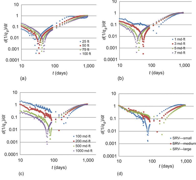
Reciprocal of Gas-Rate Derivative vs. Time. This type of diagnostic plot is used in this work to help characterize fracture parameters when multiphase flow is involved, which is always the case during the flowback period. Fig. 3 also groups the plots by network fracture spacing, network fracture conductivity, primary-fracture conductivity, and SRV size. The left part of the plots represent the time period during which the fracture is cleaning up, when multiphase flow should be emphasized. According to the curve signature of Fig. 3a, the pseudoradial-flow regime has been developed after approximately 1 year of production for the case with fracture spacing of 25 ft. For the other three cases with larger fracture-spacing values, it takes a longer time to establish the pseudoradial-flow regime. The observation from Fig. 3b is that cases with higher network conductivities reach the compound-linear-flow regime at earlier time. However, the four curves tend to merge at some point. Another item that needs special attention is that, excepting the case with 1 md-ft, the other three cases fall on the same line even during the compound-flow regime. This indicates that, after fracture cleanup is achieved, network fracture conductivity greater than 3 md-ft should be sufficient for the shale-matrix permeability used in this simulation. Fig. 3c is for cases with varying primary-fracture conductivity. In this case, after fracture cleanup, fracture conductivity greater than 500 md-ft does not show incremental benefit for this given set of reservoir and fracture parameters. Unlike the other three groups, plots in Fig. 3d illustrate distinct signatures. The simulation case with the smallest SRV reaches pseudoradial flow after approximately 1.5 years of production, while the one with the largest SRV is still in the compound-linear-flow regime after producing for 3 years.
This article, written by JPT Technology Editor Chris Carpenter, contains highlights of paper IPTC 16896, “Characterization of Hydraulic-Fracture Geometry in Shale-Gas Reservoirs by Use of Early Production Data,” by Chunlou Li, Randy LaFollette, Andy Sookprasong, and Sharon Wang, Baker Hughes, prepared for the 2013 International Petroleum Technology Conference, Beijing, 26–28 March. The paper has not been peer reviewed. Copyright 2014 International Petroleum Technology Conference. Reproduced by permission.