It would be exceedingly hard to find anyone with more experience extracting data from a fractured reservoir than Kevin Raterman.

After nearly a decade as co-leader of ConocoPhillip’s one-a-kind test site in the Eagle Ford, Raterman, a reservoir engineering advisor at the company, has had the opportunity to use just about every sort of diagnostic test.

He was the lead writer on the latest technical paper (URTeC 263) about the test site that studied “core, image logs, proppant tracer, distributed temperature sensing, distributed acoustic sensing, and pressure, which shows that not all hydraulic fractures are created equal.”

Among those, the measurements from an array of downhole pressure gauges loomed largest.

Raterman’s advice to those analyzing fractured reservoirs is to install more downhole pressure gauges to identify where fractures are draining the rock and where they are not. Those carefully placed sensors observed large pressure differences at locations as close as 45 ft apart.

“The more spatial pressure data you have, the better off you are,” he said. Pressure gauges are one of the oldest tools for reservoir analysis, and one of the more affordable. The test site plan to gather spatial data, though, significantly upped the ante. It required installing gauges in the reservoir at carefully chosen locations in what would normally be inaccessible rock.

ConocoPhillips installed 14 pressure gauges in monitoring wells around the fractured producing well, where the 15th gauge was located. Based on other diagnostic tests, the locations showed how a small number of large fractures can play a dominant role in draining the reservoir. It was part of ConocoPhillips’ exhaustive reservoir test in the Eagle Ford that was launched in the heady days when $100/bbl oil seemed like a given.

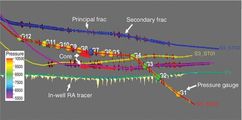
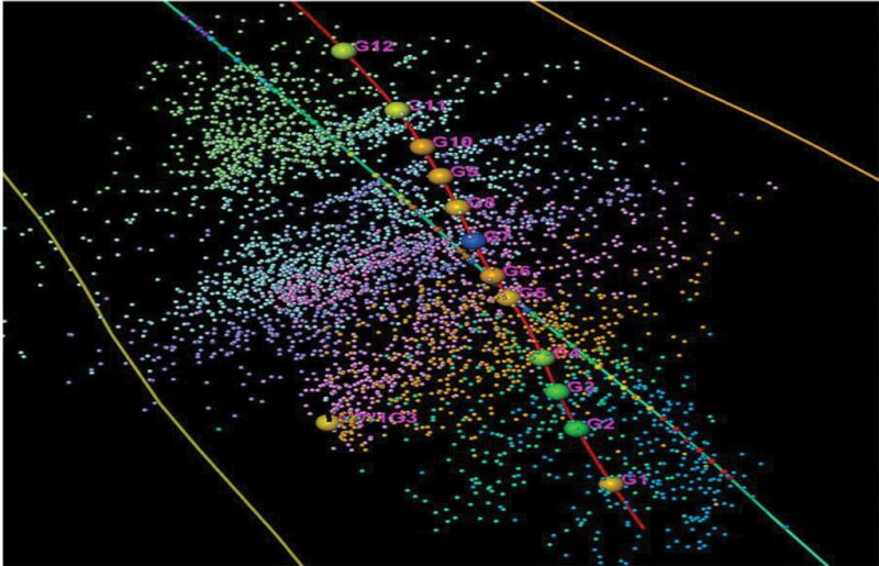
The new technical paper examined 12 pressure gauges installed in a monitoring well originally drilled for testing, which had focused on imaging thousands of feet of rock and collecting one of the largest samples of fractured core ever (Fig. 1).

The core samples were the stars of the first test site paper in 2017 (URTeC 2670034). That attracted a lot of attention because the samples contained a complex mix of large and small fractures that contradicted widespread assumptions about fracturing.

It was widely assumed that the millions of pounds of sand pumped to prop open fractures extended to a large area around the well. But at those far field locations, from 60–400 ft from the well, “evidence for well propped fractures is sparse.”

Those samples were also interesting because hydraulically fractured core is rarely collected. Coring fractured rock is costly and difficult. The ConocoPhillips team had to develop a method to collect the fragile, cracked samples.

There are limits to what can be learned from the cracks in a cylinder of rock a few inches wide. Those fracture segments are a static piece of a dynamic system.

A large hydraulic fracture in a core sample suggests there is a flow path to the well. That is like knowing there is a pipeline at one spot, but not where it goes, how much it carries, or if that changes over time.

When weighing the value of collecting fractured core vs. recording pressure changes, Raterman said: “There is a strong contingent married to the geology. They say if someone understands the rock properties on a foot-by-foot basis you are going to be able to predict the outcome of the fracturing.”

Even though the Eagle Ford test site collected an unprecedented amount of fractured core, he said it was still under-sampled. “We drilled a lot of linear feet, but based on the (reservoir) volume, the sample is minuscule,” Raterman said.

A Few Good Fractures

In an industry where companies are reluctant to pay to install a single downhole pressure gauge in a well, ConocoPhillips installed 14 in monitoring wells drilled for that purpose and built to ensure that each only measured pressure changes nearby. Multiple tests were required to choose locations likely to show both where large fractures were draining the rocks and spots with minimal production.

A chart condensed the layers of information used to identify the location of the large and the small fractures along a 2,000-ft-long horizontal well section (Fig. 2). On the chart, the black lines at the bottom that Raterman calls black tick marks are large fractures that are likely to be productive. This special class of fractures are called principal fractures.

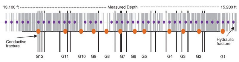
Those 19 principal fractures were among the 996 fractures identified using image logs (FMI-HD). The small ones appear as gray tick marks, which are so numerous they often meld into solid gray areas.

The primary evidence used to locate principal fractures were borehole images showing broad dark bands—a conductive zone likely due to a concentration of saline drilling mud pushed into large-aperture hydraulic fractures. The electrical conductivity of salt contrasts with the resistive rock around it.

Other clues included the few propped fractures observed in the collected core and the spectral gamma ray log showing concentrations of radioactive tagged proppant associated with the dark bands, suggesting these large fractures were well propped.

Installing the pressure gauges at those carefully chosen locations was a major challenge. First, they had to design a completion that ensured each gauge was isolated from the others, so a pressure change at one location did not alter readings down the line.

Fiber-optic pressure sensors were attached to casing at the surface. The sensors were put into the casing, which was also perforated to allow pressure gauges inside to detect pressure changes outside the well. Adding extra centralizers ensured that the cement around the casing was thick enough to create an effective barrier, and low-permeability cement further limited pressure communication. Inside the casing, composite bridge plugs isolated each sensor.

Ultimately, the value of the test data depended on placing the gauges within 10 ft of the targets. Running the casing right was critical. “Where we felt the risk was more on getting everything to TD (total depth),” Raterman said.

Pressure Signals

The value of all that time and money invested only became clear when the pressure measurements began flowing after about a year of production, which was 18 months after the first oil produced plus downtime.

Pressure-change data over time allowed the company to determine if ­production from fractured reservoirs flows from an irregular pattern of fractures draining a portion of the stimulated area. Irregular production from stage to stage is the norm. The goal was to track the differences back to the source using far-field pressure gauges measuring where production is strong, and spots where it is not.

“Depletion continued at all gauge stations over a 3-year period. The degree of depletion, however, remained quite localized and variable,” the paper said.

For example, the flowing pressure difference between one principal fracture (G7) and its nearest neighbors grew to as high as 5,000 psi as that active fracture lowered the pressure by draining the area. At the other extreme were locations for gauges chosen opposite where perforation guns failed to fire (G10, G8) and no principal fracture were detected.

As a result, only half the gauges “demonstrated an effective connection to the well” based on the pressure drawdown.

The variations argued that the principal fractures that were predicted using other testing really were the primary production source. The question remained, could they be sure that drainage by 2% of the hydraulic fractures represented the largest share of the production?

“We tried to find a correlation of the pressure data to every variable we could think of. The only things we found that it was correlated with was proximity of the gauge location and the black tick marks” marking principal fractures, Raterman said.

Based on the work, he said, “we feel strongly” a high-quality image log can identify major productive fractures.

Secondary Considerations

The company also had to account for the small secondary fractures—the gray tick marks—which also posed a problem: “How are these hydraulic fractures connected to the producer and do they contribute to production?” Raterman said.

To address it, they analyzed fiber-optic distributed-temperature sensing to measure the temperature drop near the wellbore after cooler fluids from the surface were pumped into the hot rock, and also how fast the reservoir warmed afterward.

They concluded that many of the sampled secondary fractures likely connect to the producer. By including these observations into a pressure-history-matched reservoir model, they predicted that secondary fractures represent roughly 40% of total production.

“Production estimates were made on the premise that the entirety of hydraulic fractures operate as a system, driven by the idea that they all contribute,” he said.

The simplified model assumes that the majority of production moves to the well via the principal fractures, which extend the farthest and drain the most based on the pressure drop measurements.

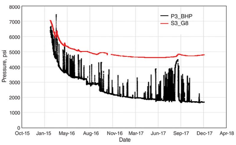
Pressure sensors showed that fracture flow trends sometimes change over time. During the first year of pressure measurements, there were rapid pressure declines near one of the biggest fractures, measured by sensor G7, and strong production (Fig. 3).

Then there was a curious change. The pressure started rising, moving up 400 psi. It appeared that while oil and gas production continued near the pressure gauge, pressure was building because the amount flowing to the well was shrinking. During that period, the oil production rate dropped 90%. The paper said this may be due to “the detrimental effect of fracture failure.” This observation could mean there is value in refracturing to reopen shrinking flow paths.

Impossible and Required

A colleague of Raterman’s, Dave Cramer, also an engineering advisor at ConocoPhillips, describes him as a “bright and skeptical guy,” adding that for Raterman “it is an impossibility to capture and predict all the nuances going on in a frac treatment.”

After that, Cramer mentioned details about completions that could significantly affect fracturing and future production—such as the erosion rate in perforations used for fracturing.

The fact that beyond a small group of completion experts most people doing modeling would not consider how a high-pressure flow of water and sand would widen a perforation and alter fracture development argues that it likely is impossible to consider every significant variable when modeling hydraulic performance. Even if such a model existed and the data was available, the computing power and time needed to run it would be prohibitive.

The exploration and production business requires models based on meaningful, measurable data points that make use of what has been learned about the complexities of fractured reservoirs.

“The practical necessity is that this complexity must be translated into the reservoir modeling domain such that spatial damage can be adequately delineated and long-term production predicted,” the paper said.

The ConocoPhillips paper did not recommend a model. It did evaluate four models to see how well they dealt with the variations of the drainage rates due to irregularly spaced fractures. The result was not an endorsement of any one approach, though the paper said only two of them “adequately approximated the far-field pressure data.”

After this evaluation, the paper suggests ConocoPhillips began taking modeling results with a grain of salt when planning wells.

“Prohibitions based on fracture modeling were largely supplanted in favor of experimentation: A tacit recognition of the fact that the observed outcome was unpredictable utilizing existing tools,” the paper said.

The simplest model performed poorly because it was unable to incorporate variable production among the fractures.

“Everything is too homogeneous and uniform to match the pressure data in the far field,” Raterman said.

A second model performed better because it allowed the company to remove the assumption that all of the fractures are identical. However, the limited number of predictions that matched the well history indicated it was not ideal.

The third example was a hybrid, widely used workflow at ConocoPhillips. It combined the best-selling fracture modeling program, Gohfer, plus an internal workflow to introduce fracture properties and how they are likely to change over time, into the reservoir model.

The results predicted the fracture height that was greater than observed, and like the second example, it assumed each fracturing cluster created one fracture, which was not the case. “As you might guess, it misses on some counts,” Raterman said (Fig. 4).

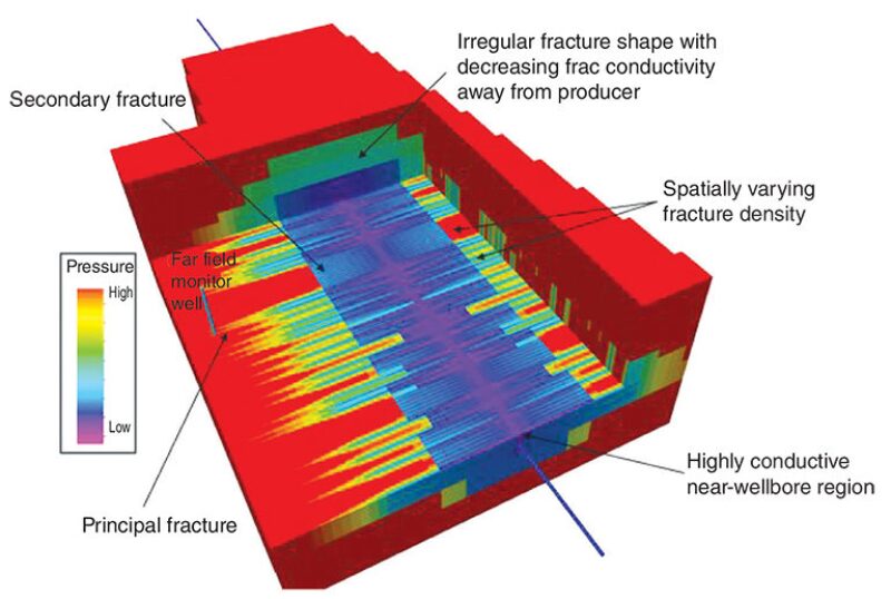
The paper said it tended to “under-predict” variations in the fracture geometry and over-estimate fracture-height growth. The critique suggests that combining a planar fracture model and other data in the hope of getting a more accurate view of a specific well can have unintended consequences.

The fourth model allowed the inputs to vary along the lateral and the paper said that when the history match test was done, “multiple realizations were deemed acceptable” for the independent variables tested.

The paper did not offer comparable history-match numbers for all four models but concluded: “Only phase two and phase four models adequately approximate the far-field pressure data. This outcome establishes variable effective fracture geometry as a necessary condition for history matching such data,” said the paper, adding that, “Whether this establishes a necessary and sufficient criterion can be debated openly.”

The Model Muddle

The production decline rates that appear in ConocoPhillips’ financial reports are calculated “empirically,” Raterman said. In other words, production is predicted using statistical analysis of production data and decline-curve techniques, not a model based on the physics of reservoir flow.

That is a workable response to the shortcomings of models of unconventional reservoirs. However, what works for financial reports, which rely on historical data, is little help to those needing a tool to digitally evaluate new well designs and completions. Realistic simulations are required because trial-and-error testing in the ground is so expensive.

The agenda at the recent URTeC conference showed that there are plenty of people working on creating working models for fractured reservoirs, and plenty of skeptical questions raised about the analysis. Near the end of an afternoon-long session analyzing the Permian Fracturing Test Site results, three speakers offered predictions based on rate-transient analysis.

In the middle was Jorge Acuña, a reservoir engineer for Chevron, whose predictions were based on his rate-transient analysis method. His expectations varied from those who presented before and after him, though they shared a similar database from the Fracturing Test Site I in the Permian. He said expectations vary because modelers from “different companies looking at the data look at the data differently.”

Modelers have varying views of the key factors driving reservoir performance. For example, some say the data indicate there are “enhanced permeability regions” within reservoirs that fade over time. Acuña says those are not a significant variable.

He explains his method by saying: “If the rock is broken in many pieces of different sizes, it is possible to explain the behavior of unconventional wells as the combined effects of all those fragments acting together.”

Underlying this fracture network model is fractals—a branch of math he defines as complex patterns that are self-similar across different scales. These may behave in non-intuitive ways and may offer a way of dealing with irregularly fractured, ultra-tight rock that is altered unpredictably by hydraulic fracturing.

For example, wells with high initial production, large initial decline, and high gas/oil ratios are the result of fragments initially working similarly, and then evolving at different speeds to reduce oil production and push up the gas/oil ratio. Smaller blocks will change faster than larger ones (URTeC 2876208).

Long or Short?

Tom Blasingame, a Texas A&M University professor whose work on rate-transient analysis goes back to the mid-1990s, said the problem became far more difficult after the industry shifted from drilling vertical conventional wells to fracturing multistage horizontal wells. The number of variables surged with the number of stages, each of which might add fractures, or not.

“With horizontal wells with multiple fractures the process becomes inherently non-unique because those fractures had to be accounted for,” he said.

The possible answers could range from shorter fractures in a relatively more permeable system or longer fractures in a less permeable system. The first option argues for tighter well spacing, while the second suggests closely spaced wells would lead to destructive interference during fracturing.

While the ConocoPhillips test site found that most of the productive fractures clustered close to the well, there were exceptions, including “some fractures that grew out 1,000 ft or more.” That data suggest there can be physical evidence for both nonunique answers.

One way to narrow the answer set is to do a diagnostic fracture injection test (DFIT). This in-well test uses a small-volume injection to test rock properties, including permeability. That result can reduce the uncertainty for those deciding what numbers to input in the RTA calculation.

But there are questions about the accuracy of DFITs results in some cases, particularly on shale gas wells. That led seven large operators and a service company to form a joint-industry project to determine how to accurately do and interpret DFITs tests, the results of which were presented at the conference (URTeC 123).

The lead author of that paper, Mark McClure, chief executive officer of ResFrac, a company developing a ­fracturing-based reservoir model, said the process used to develop that method was based on multiple sets of field data from supporting companies.

He has also experienced how disagreements among modelers can get passionate, and personal. The speakers at the URTeC session who had done RTA analysis faced tough questions about the flow regime they had chosen for their analysis.

Models often assume the reservoir is in a period of linear flow—the time when the fractures all produce independently of one another, Blasingame said. The reality can change based on the fracture geometry or the presence of multiphase flow.

“Why bog you down with all this detail? Because almost every (simplified) analysis method being proposed has linear flow as its basis,” Blasingame said. This matters because “if this condition is not met, then all of the results and interpretations derived from this are, well, not right either,” he said.

His advice to petroleum engineers is to gather more downhole pressure data.

Raterman advised anyone feeling confident about modeling results to do a reality check. “Internally I tell people to collect data before you make assumptions in the model because you are liable to be wrong,” he said.

Taking a New Look at Microseismic

Microseismic testing is supposed to be able to show where hydraulic fracturing creates productive fractures, but results from a ConocoPhillips’ test site in the Eagle Ford suggest otherwise.

For years, microseismic has been used to monitor fracturing based on the assumption that clusters of events—the sound of small faults shifting—are an indication of where hydraulic force is quietly opening fractures in the tight rock.

The first of two reports on testing at the ConocoPhillips’ site concluded that there is “no direct statistical relationship between sample hydraulic fracture density and microseismic event density,” based on fractured core collected away from the well (URTeC 2670034). The second paper added that microseismic data has little statistical relationship between the microseismic events and the locations of productive fractures, based on data from downhole pressure gauges (URTeC 263).

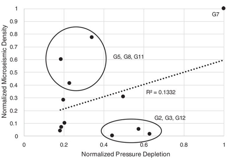
“No correlation between normalized pressure drawdown and normalized microseismic density was determined,” the second paper said.

“Based on the pilot data, the proper use of microseismic data appears limited to describing the spatial extent of the stimulated reservoir volume (SRV). Using microseismic activity as a proxy for effective permeability seems to be largely unsupported, it said.

Fractures opened by hydraulic force do not create a sound but the thinking has been that the microseismic events, shown as colored dots, show where fracturing is occurring (Fig. 1).

In its second paper, ConocoPhillips used pressure gauges in monitoring wells to confirm that a small number of large, well-propped fractures were responsible for much of the production. The pressure drops near those principal fractures did show significant production. But the connection with microseismic activity was hit or miss.

A gauge placed at the most productive spot with the largest pressure drop was in an area with a dense cluster of seismic events (Fig. 2). Three gauges showing limited production were in areas with many events, and three gauges showing large pressure drops were in spots with little microseismic activity.

The paper did say microseismic can offer a picture of the total area stimulated, including a large fracture extending 1,000 ft or more from the well, but said a really long fracture is not likely to be productive that far out.

Using Fractals to Define Fractures

A model for a fractured reservoir based on fractals is not too hard for engineers to understand, according to Jorge Acuña, a reservoir engineer at Chevron who created one because “it is much easier than some of the models being now proposed.”

That may be true. But a model based on a branch of math not likely covered in petroleum engineering classes is likely to raise questions.

Fractals offer a way to address a problem facing anyone modeling a fractured reservoir—production and fracturing vary significantly from well to well.

Acuna’s paper offers a way for modelers to introduce some order into this chaos, with a method to define the “characteristic flow pattern.” Reservoirs that share the same characteristic flow volume should exhibit “the same hydraulic behavior.”

The method was the product of research dating back to when he was in graduate school.

“A fractal fracture network has a particular flow behavior that I studied for my thesis that is also evident for me in unconventional wells,” he said.

In this case, a “fractal network is just a group of rock fragments with sizes distributed according to a power law,” Acuña said. Evidence of that statistical relationship goes back to work in the 1940s showing that the size relationship among rock fragments created by crushing follows a power law distribution. Later researchers also identified a power law distribution in rocks broken by weathering, explosions and impacts.

Based on this concept and outputs of this rate transient analysis method, he said it is possible to define the “property that defines fluid flow behavior for complex networks of fractures.”

He suggests searching online for “fractals and fragmentation” or “rock power law fragmentation.” Details about his method are in his 2018 paper, Straightforward Representative Fluid Flow Models for Complex Fracture Networks in Unconventional Reservoirs (URTeC 2876208).

Looking for more information on developments in hydraulic fracturing? Consider attending the Hydraulic Fracturing Technology Conference and Exhibition, 4-6 February 2020 in The Woodlands, TX USA.