Financial reports have long lumped shale acreage like cuts of meat, with tier 1 for the best reservoir rock, and tiers 2 and 3 ranked as lower quality.
Tier 1 is rated superior to the lower tiers based on a handful of geological measures related to the oil in the ground and the ability to stimulate flow with fracturing.
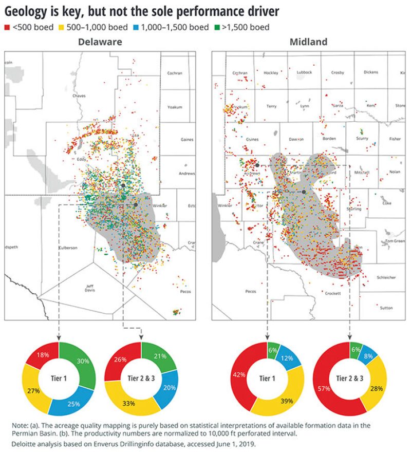
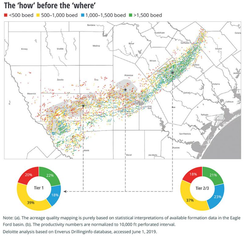
Production tells another story. A recent study by the energy advisory arm of Deloitte of 35,000 wells in the Permian Basin and Eagle Ford found that production in regions outside tier 1 in those basins are not that different.
“We are starting to challenge that general notion that just investing in established tier 1 acreage drilling a longer lateral, pumping more proppant,” ensures wells that are both productive and profitable, said Tom Bonny, a managing director for Deloitte.
In the Eagle Ford shale, the breakdown in wells based on early production showed little difference between the tiers. Tier 1 wells had a slight edge in wells producing more than 1,500 BOE/D, but was also a bit higher in the percentage of wells at 500 BOE/D or less.
In the Midland Basin, the pie chart for tier acreage showed tier 1 outperformed lower tiers at both the high and low end.
The differences at the high end were relatively small. In the lowest quartile, the percentage of tier 1 wells was significantly lower but 42% of the tier 1 wells were in the bottom quartile, pointing to another problem highlighted by the data—many shale wells are not that productive. In this story, production is based on a 180-day measure that is adjusted as if it were from a 10,000-ft lateral, unless otherwise noted.
The message in the study is that reservoir rock quality matters, but even in what passes for good quality shale rock, getting oil out depends on where the well was located and how it was drilled, fractured, and produced.
“Rock is important, but a good rock without a good design is of less use,” said Anshu Mittal, an associate vice president for Deloitte.
An average of the splits in the Deloitte pie charts are roughly in line with a rule of thumb offered years ago by George King, now a principal with GEK engineering, who said that for every 10 shale wells, there a couple of bad ones, a handful of marginally profitable performers, and a few strong wells that justify the effort.
What was once a wry observation back when oil prices were $100/bbl now sheds light on a pressing problem after the 2014 price crash forced companies to focus on increasing well productivity.
Operators reacted to that by driving down costs—often by reducing fees for services—and paying more to drill longer laterals and pump more sand.
During those years, the growing use of data allowed those inside the business, and outside, to critically consider the methods used to produce more oil and gas, and whether a well that produced more was worth what was spent to deliver it.
Results have improved, but Deloitte’s data, going back 10 years, show there are still a lot of low performers.
“Almost 60% of the oil and gas wells drilled in US shales since 2010 had productivity (IP 180 days) of lower than 750 BOE/D. Despite notable design improvements, the share of such wells has remained nearly 50% in the past 4 years,” the report said.
Also over the past 2 years, the shares of many large shale players have plunged as investors backed away from companies that failed to deliver the cash flow needed to fund their operations and finally offer a return on the billions of dollars invested.
Deloitte said companies need to rebuild credibility with investors by avoiding “selective reporting of parameters and present a comprehensive picture” acknowledging the problems, and discussing how they are being addressed.

Return on Capital
A useful definition of the best place to drill can be found on an old web page from Kimmeridge Energy: “It is simply the area of the play where the wells produce the highest return on the capital employed.”
The web page, dated 2012, assumed that the best returns were going to be in the core area—another term for tier 1. “The vast superiority of investment returns for core acreage vs. fringe acreage makes early identification and leasing of the core critical for companies in any new shale play.”
This geologic focus led to record prices per acre during the peak of the shale boom, when earning reports regularly showed initial production rates rising year after year.
Good rock still matters, but the industry has learned it varies in unpredictable ways over short distances.
Companies still consider the geological measures used to build Deloitte’s tier maps—gamma ray, neutron porosity, formation thickness, deep resistivity, bulk density. Some are adding tools, such as geochemical testing, because sometimes what looks like a promising reservoir on those traditional measures, lacks the permeability to meet those expectations.
Rules of thumb for completions are also in question. For years, pumping more sand and fluid appeared to be a sure way to increase well productivity, but not lately.
“Over the past 3 years (2016–2018), the industry’s productivity was flat despite a 25% increase in proppant and fluid loading,” the report said. Wells with big fracturing jobs can produce more, but the amount of increase may fail to justify the expense.
The data Deloitte analyzed showed many such instances where the added production of a well was not economic. In those cases, Bonny said, “maybe that was not always the right decision.”
The analysis of the well database from Enervus (formerly Drillinginfo), showed that when it comes to completions, sometimes less is more. Many of the top-performing wells had relatively short laterals—perforated intervals from 4,000–6,900 ft.
Deloitte found little connection between proppant quality and production. The industry has already acted on that conclusion, dumping higher-cost ceramic proppant in favor of sand, and then shifting to nearby sources to save the cost of shipping from distant mines.
And operators are looking for other ways to improve productivity. The numbers show a growing range of fracturing design parameters tried over the past 3 years, “reflecting that experimentation is on the rise,” Deloitte said.

Getting Granular
“There’s not a step change that you suddenly cross, a 1-mile distance and all of a sudden the reservoir completely changes from tier 1 to tier 2,” said Jeff Yip, a petroleum engineer for Chevron.
Previously he was on a team at Repsol that created a model using advanced data analysis to identify potential drilling locations in a large Canadian play based on geologic, technical, production, and economic data. “What you are seeing is the emergence of a more granular approach,” he said.
Data-driven analysis of geological and economic information highlights exceptions to generalizations, like tiers. For engineers, areas are generally defined by type wells. Those are an assessment of the estimated ultimate recovery (EUR) for wells in an area based on geological, production, and economic data.
Accurate productivity estimates are critical because operators cannot afford trial-and-error reservoir development.
“In my discussions with operators (a limited sample), I find that they do construct type wells by area. These areas appear to be large, and, within an area, there can be significant variations in estimated ultimate recovery,” said John Lee, a petroleum engineering professor at Texas A&M University known for his work in reserves estimation.
“Careful statistical analysis can identify areas with significantly different values of mean or average EUR within the area after normalization for lateral length and completion design,” Lee said.
There is a limit to how granular a type well can be. An accurate estimate requires data from at least 50 producing wells. In addition to production data, it should include details such as the propped hydraulic fracture length and, to a lesser extent, fracture spacing, Lee said.
“The number of wells included in the sample is quite important; otherwise, the results can be completely misleading,” Lee said.
The risk of small sample sizes is not debatable. Still, exploration teams are paid to accurately predict the most productive spots to drill, even in areas where the available data fall far short of that standard.
The Duvernay in western Canada is one of those plays with great potential based on the wells drilled and fractured, but those data sources are few and far between.
Exploration teams evaluating expanses of undrilled acreage must augment that data with other sources, such as geological data from older vertical wells drilled though the target zone.
“I think you are seeing every company trying to develop their own multivariate model tying together things they believe should impact production,” in the Duvernay, Yip said. There is no standard approach. He said these “models are all based on hypotheses, and each company is hoping theirs is correct.”

Lumpers vs. Splitters
In the world of play analysis, there is tension between “lumpers and the splitters,” Yip said.
Lumpers are looking for a useful generalization, like tiers or type wells covering a large area. Splitters are the ones saying the variable nature of these formations means there are zones within large areas, where wells will diverge from the mean.
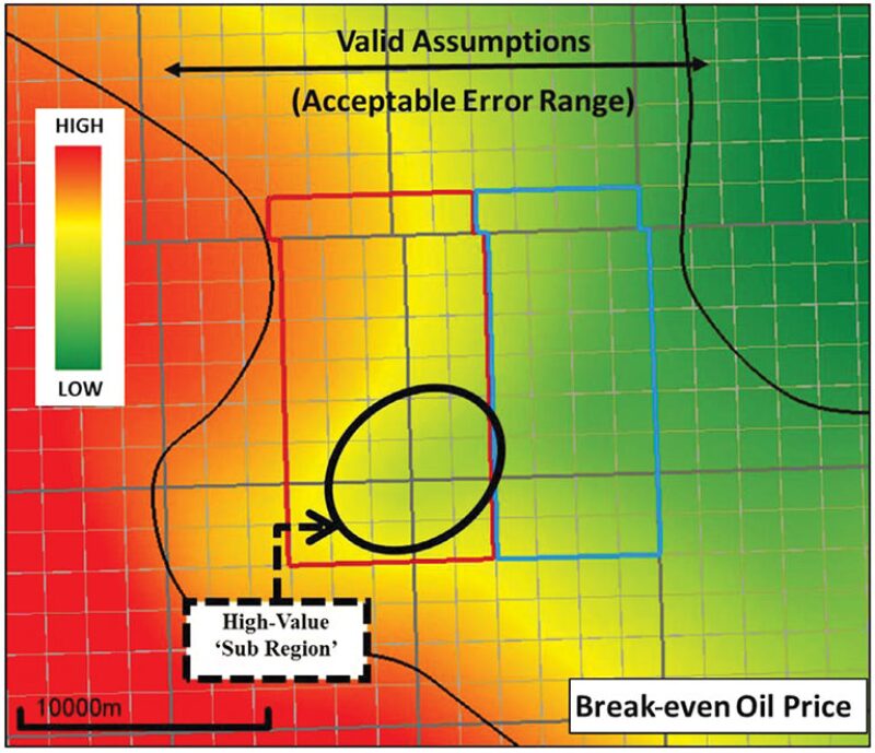
An example of this push and pull is a brightly colored heat map based on modeling done by Yip and others in 2018, while they worked at Repsol (SPE 189815). It was based on data from a small number of scattered horizontal wells plus geologic data from older vertical wells drilled through the target zone. That, plus economic data—such as the potential value of gas production or the cost of developing wells and gathering gas—was run through advanced statistical analysis.
Using a multi-variable statistical model, they combined geologic maps showing changes in the geologic quality on a mile-square grid, as well as the richness of the likely production, as measured by the ratio of more valuable condensate to dry gas in the ground.
The result was a map predicting the range of break-even oil prices for well locations within an area covering hundreds of square miles.
A circle near the middle highlights a promising prospect that likely would have been dismissed using older methods, which predicted better results in a large area to the right of the circle, in the blue rectangle.
“Each box was originally represented by a single average type curve, despite all the variability in the reservoir. Based on the break-even oil price, the blue region was more economically attractive than red, and actually red was at risk of not being drilled at all,” he said.
While the analysis led the company to consider drilling within the circled target in the red zone, Yip does not know what happened after he left.
This analysis hinges on using AI to maximize the value of a thin database, which has its risks.
“For a small sample, the mean of the sample may be significantly different from the mean of outcomes from the entire population in an area, so I would be very cautious about subdivisions of resource plays that are too small,” Lee said.
The Repsol modeling paper acknowledges the risk. A black arrow at the top of the map defines the edges of the area where the level of uncertainty in the data is manageable. Beyond that line are many miles of prospects where the break-even price appears more attractive than the prospect identified.
Those areas were ruled out because they are beyond where they had “sufficient confidence in our multivariate model,” and geologic evidence suggested the liquids content would be lower than predicted, Yip said.
Still the map made those fringe areas look tempting. “The beauty of a model is that it lets you extrapolate,” Yip said, adding, “The danger of a model is that it lets you extrapolate.”


