

Explaining Traditional Engineering Models
It is a well-known fact that models of physical phenomena that are generated through mathematical equations can be explained. This is one of the main reasons behind the expectation of engineers and scientists that any potential model of the physical phenomena should be explainable. Explainability of the traditional models of physical phenomena is achieved through the solutions of the mathematical equations that are used to build the models. Explanations of such models are achieved through analytical solutions (for reasonably simple mathematical equations) or numerical solutions (for complex mathematical equations) of the mathematical equations. Solutions of the mathematical equations provide the opportunities to get answers to almost any question that might be asked from the model of the physical phenomena.
Solutions of the mathematical equations are used to explain why and how certain results are generated by the model. It allows examination and explanation of the influence and effect of all the involved parameters (variables) on one another and on the model’s results (output parameters). In general, this is the definition of the engineering approach to problem solving. Therefore, results of the physical phenomena that are based on mathematical equations (no matter how simple or complex) can be explained in detail.
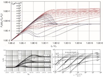
Fig. 1 shows the Fetkovich type curve, including early-time (driving from transient flow equations) and late-time curves (boundary dominated flow, Arp’s decline curves). Equations 1 and 2 are used for this series of type curves.
Equation 1 .............. qDd = qD[ln(re/rwa)−½]
Equation 2 .............. tDd = tD/(½[(re/rwa )2−1][ln(re/rwa)−½])
Dimensionless rate (qD) and time (tD) used in Equation 1 and Equation 2 are defined by Equations 3 and 4, respectively, in the context of well-testing domain.
Equation 3 .............. qD = (141.2 q μ B)/[k h (pi−pwf)]
Equation 4 .............. tD = (0.00633 k t)/(ϕμ ct rw2)
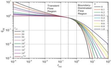
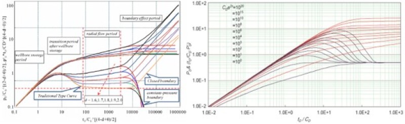
It can be clearly seen that the curves in Fig. 1 are very well-behaved (continuous, nonlinear, of a certain shape that changes in a similar fashion from curve to curve). The reason behind the well-behaved characteristics of these curves is the mathematical equations that were used to generate them. All type curves that have been historically generated in the petroleum industry are very well-behaved because they all are developed using the solutions of the mathematical equations. Fig. 2 demonstrates two more examples of such well-behaved type curves.
This means that traditional, mathematics-based models of the physical phenomena are explainable. Physical phenomena that are developed using mathematical equations are explainable by performing several types of analyses of the mathematical equations. The following are four ways of explaining physical phenomena models that are developed and solved using mathematical equations:
- Identification of the influence of each parameter (variable) in the mathematical equation, also known as key performance indicators (KPIs)
- Single-parameter sensitivity analysis
- Multiple-parameters sensitivity analysis
- Type curve generation
Performing such analyses can provide the required explanation of any question that might be asked regarding why and how certain outcomes are generated or certain forecasts and predictions are made based on the solutions of the mathematical equations that have been used to model the physical phenomena. Figs. 1 and 2 demonstrate examples of type curves that are generated through the solutions of certain mathematical equations.
Explaining Models of Physics Developed by AI and Machine Learning (XAI)
A recent article that was published in Forbes mentioned: “Many of the algorithms used for machine learning are not able to be examined after the fact to understand specifically how and why a decision has been made. This is especially true of the most popular algorithms currently in use—specifically, deep-learning neural network approaches. Explainable AI (XAI) is an emerging field in machine learning that aims to address how black-box decisions of AI systems are made. So far, there is only early, nascent research and work in the area of making deep-learning approaches to machine learning explainable.”
This article was written in July 2019. It demonstrates that systems and models mimicking human-level intelligence (nonengineering-related problems) that have been developed using AI and machine learning have major issues with explaining how this technology predicts, forecasts, or makes decisions. The type of applications of the AI and machine learning that is the reference of this article, as well as many other recent articles about XAI, are mainly related to the application of this technology to nonengineering-related problems. When it comes to engineering applications of AI and machine learning, “how and why a decision has been made” becomes far more important than when this technology is used for nonengineering-related problems. Therefore, what today is being called XAI has been a major issue when this technology started to be used in petroleum engineering in early 1990s.
It is interesting to note that explainable predictive models developed using AI and machine learning were developed by Intelligent Solutions in early 2000s. These XAI models are part of the application of this technology in petroleum data analytics. As has been mentioned, the main reason behind the research and development of XAI, which took place much earlier, had to do with the fact that, once this technology is applied to engineering-related problem solving, explainability of the models become a critical issue to scientists and engineers.
The main reason behind calling the predictive models that are generated using AI and machine-learning algorithms “black box” has to do with the fact that these algorithms do not model the physical phenomena using mathematical equations. When it comes to the engineering application of AI and machine learning, the black-box characteristics of such models will cause serious problems for scientists and engineers. Many traditional engineers who have a negative view of this new technology usually use the term “black box” to deny the contribution of this technology to the future of engineering problem solving.
One of the major contributions of petroleum data analytics that has been developed during the past 3 decades at Intelligent Solutions and West Virginia University is the creation of transparency for the so-called black box of the predictive analytics. Because petroleum data analytics is a purely physics-based technology through avoidance of any mathematical equations, and generates purely data-driven predictive models, it develops explainable predictive models. The objective of this article is to demonstrate the XAI modeling of petroleum data analytics. This demonstration will be explained through KPIs, sensitivity analysis, and type curves.
KPIs
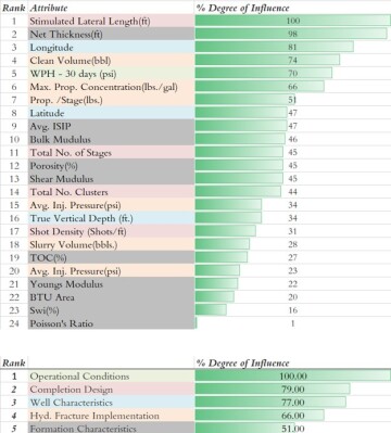
Predictive models developed in the context of petroleum data analytics can provide a tornado chart to demonstrate and rank the contribution of all the input parameters that were used to develop (train, calibrate, and validate) the predictive model. Fig. 3 shows a tornado chart generated from the data-driven predictive model developed using shale analytics for a Marcellus Shale field in southwestern Pennsylvania. The data-driven predictive model that was developed for this reservoir- and completion-engineering-related problem used 24 different field measurements. The output of this predictive model was 30-day cumulative gas production from each well in this field.
The KPI tornado chart of this data-driven predictive model shows that, on the average, the operational conditions in this field plays the most important role in controlling the first 30 days of gas production. It then is followed by attributes associated with completion design, well characteristics, hydraulic fracture implementation, and finally the formation characteristics. In Fig. 3, the background color of each of the attributes (input parameters) identifies the category to which the input parameters belong.
Sensitivity Analysis
One of the major techniques that can be used to explain the behavior of a model is sensitivity analysis. The predictive analytic models that are developed in the context of petroleum data analytics include several input parameters that are used to build a purely data-driven (field measurement), physics-based model of the given output. In the context of reservoir engineering, let’s consider building a predictive shale analytics models that uses reservoir characteristics as well as completion design and implementation (as part of other input parameters) to model the well productivity index.
Sensitivity analysis of these particular predictive shale analytics models, which will be explained in the following three steps, can be applied to each well that has been used to build the AI-based model. The sensitivity analyses that are demonstrated in the following sections can also be applied to specific sectors of the reservoir (in the case of shale assets, they can be applied to each pad that includes a series of shale wells) that would include a certain numbers of wells and also can be applied to all the wells in the entire field.
Step One: Single Parameter Sensitivity Analysis. Data from approximately 250 wells in the Marcellus Shale was used to develop this shale predictive analytics model. Once the model development was completed, in order to check the model behavior, the model output is analyzed as a function of modifying each input parameter to see if the results of such analyses makes engineering (physics) sense. In other word, the idea is to be able to explain the AI-based model behavior.
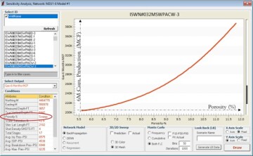
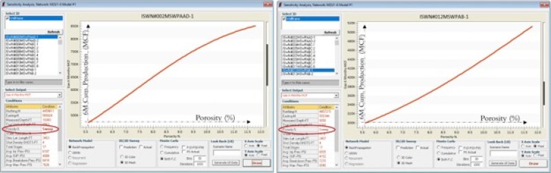
As it is shown in Fig. 4, first a specific well is identified and all the values of each parameter from this specific well that was used to build the predictive shale analytics model are demonstrated. Then one of the input parameters is selected, which is porosity in this figure. Obviously, this particular well has a specific porosity value that has been measured and then used as part of the entire data set to build the predictive shale analytics model. The purely data-driven (field measurement) model that has been developed for this field in the Marcellus Shale has proven to provide good output (6 months cumulative gas production) based on this specific value of porosity.
The question is what would happen to the model output (6-month cumulative gas production) as the value of the porosity for this specific well is modified. Keeping all other input parameters constant, the value of the porosity is changed from minimum to maximum in 100 pieces. What would be the well productivity (model output) for each new value of the porosity, while all other parameters remain constant? Fig. 4 shows the behavior of this predictive shale analytics model. This predictive shale analytics model explains that the hydrocarbon production of this particular well will increase if the porosity of the formation increases.
From a petroleum-engineering point of view, this makes perfect sense. This process can be repeated for each well in this field. Examples of two more wells in this field are shown in Fig. 5. In general, the behavior of the model is very much the same. As the porosity of the formation increases, so does the well hydrocarbon productivity.
Given the fact that all other input parameters are different for each of the wells in the field, the detail shapes of the increasing productivity curve are different from one another. From a physics point of view, this also makes perfect sense. What is very important to note is the fact that no specific mathematical equation (or predetermined correlation through equation-based data) was used to develop this predictive shale analytics model.
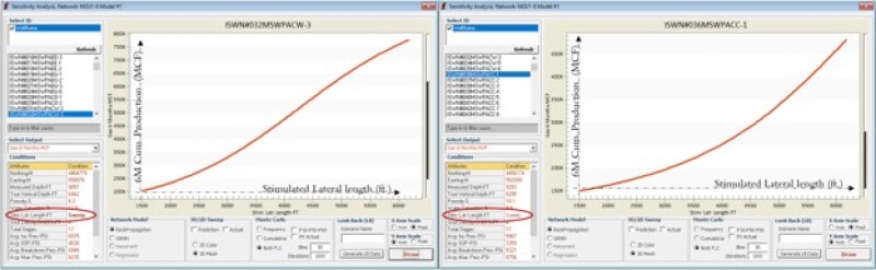
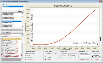
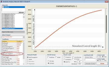
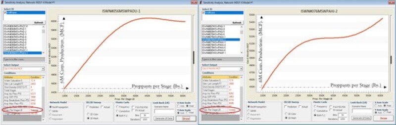
Figs. 6 through 9 repeat this analysis for stimulated lateral length and proppant per stage for multiple wells in this Marcellus Shale. The model behavior for all these wells and parameters makes perfect sense from a physics point of view. This is a good example of XAI in shale analytics.
Step Two: Double Parameters Sensitivity Analysis. Analyzing the sensitivity of two parameters simultaneously, instead of a single parameter at a time, will result in a 3D figure. As shown in Fig. 10, modification of the productivity of an identified well is explained as a function of modification of two reservoir characteristics, porosity and initial water saturation. While the AI-based model has generated the productivity of this specific well, it is explaining how the well productivity may change as a function of the modification of these two particular reservoir characteristics while keeping all other input parameters constant.
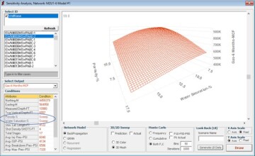
It is interesting to note that the explanation of this predictive shale analytics model makes perfect physics sense because it is explaining the way the well productivity will increase as porosity of the reservoir increases while the initial water saturation decreases. Again, it is important to note that (a) the same type of general trend (an increase of well productivity as porosity increases and initial water saturation decreases) takes place for every single well in this field and (b) no mathematical equations were used to generate any data for the training, calibration, and validation of this predictive shale analytics model.
Step Three: Multiple Parameters Sensitivity Analysis. As the sensitivity analysis of the number of input parameters increases to more than two parameters, providing figures with multiple dimensions will no longer be possible. The most common way of performing sensitivity analysis for multiple input parameters (more than two) is Monte Carlo simulation. Monte Carlo simulation has no limitation on how many input parameters can be used in order to perform multiple-parameters sensitivity analysis.
The shale predictive analytics model is used as the Monte Carlo simulation’s objective function. Once the number of parameters for the sensitivity analysis are identified, then the process can be started. In the example shown in this section, four parameters (porosity [%], initial water saturation [%], stimulated lateral length [ft], and proppant per stage [lbm]) have been identified for sensitivity analysis.
Once the number of parameters for sensitivity analyses has been identified, then performing Monte Carlo simulation requires the following three steps:
- Identify of the type of distribution for each parameter (e.g., uniform, triangular, Gaussian)
- Identify the number of times that the simulation’s objective function must be executed (the shale predictive analytics model, in this case) to generate the results (model output—here: well productivity)
- Identify number of bins to demonstrate the distribution of the well productivity as a function modification of all the identified input parameters
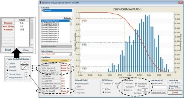
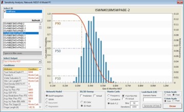
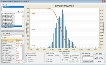
The three steps are identified in Fig. 11. Results of the multiple parameter sensitivity analysis for three of the wells in this field are shown in Figs. 11, 12, and 13. In these analyses, four parameters (porosity, initial water saturation, stimulated lateral length, and proppant per stage) were used to demonstrate the sensitivity of each well’s productivity to their modifications, while all other input parameters for each well were kept constant. The blue bar chart shows the distribution of the well productivity as a function of modification of these four parameters, and the red curve shows the summation of the distribution.
Using the red curve, P10 (almost the highest productivity of the well), P50 (almost the average productivity of the well), and P90 (almost the lowest productivity of the well) can be identified for each particular well as a function of modification of the parameters that are used for the sensitivity analysis. Characteristics of the blue bar chart and the red curve explain the physics of the shale predictive analytics model in detail for each well in this field.
Type Curves
As mentioned previously, type curves that are generated using mathematical equations are very well-behaved (continuous, nonlinear, of a certain shape that changes in a similar fashion from curve to curve). Fig. 14 demonstrates a few more examples of type curves that have been generated in reservoir engineering. The question is: What is the main characteristic of a model that is capable of generating series of well-behave type curves? The immediate, simple answer to this question is: The model that is capable of generating a series of well-behaved type curves is a physics-based model developed by one or more mathematical equations. The well-behaved type curves that clearly explain the behavior of the physics-based model are generated through the solutions of the mathematical equations.
The next question then would be: What if it can be shown (and proven) that the model that has generated the well-behaved type curves has not been developed using any mathematical equations? What if this model is purely data-driven (field measurement)? Then the answer that would make sense would be: (a) Generation of these well-behaved type curves proves that the data (field measurement) that was used to build the purely data-driven model reasonably represents the physical phenomena that was being modeled, (b) the data-driven predictive model can be clearly explained, and (c) the technique that was used to develop such model must be a scientifically solid technology.
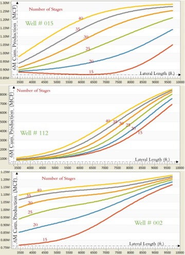
The main characteristics of the well-behaved type curves is the explainability of the model that has generated them. Figs. 15 and 16 are good examples of explaining the model that has developed them. Fig. 15 includes three series of graphs/type curves. These type curves have Stimulated Lateral Length (ft) as their X axis, and 6-Month Cumulative Gas Production (Mscf) as their Y axis. Each of the curves in a graph represent the number of hydraulic fracturing stages that are used during the completion of the well. There are six curves in each graph. Each of the graphs explains the behavior of a specific Marcellus Shale well in southwestern Pennsylvania. The six curves in each graph show how each well’s productivity changes as a function of stimulated lateral length (ft) (from 3,000 to 10,000 ft) and the number of stages (from 15 to 40 stages). The three wells that are shown in Fig. 15 belong to three different pads in three different locations in this specific Marcellus shale asset.
XAI Model for Unconventional Reservoir—Shale Analytics
Shale analytics is the engineering application of AI and machine learning in unconventional reservoirs. During shale predictive analytics, the data-driven models that are developed for completion and production optimization are based purely on field measurements. In shale analytics, use and incorporation of any types of mathematical equations are avoided because of the lack of realistic understanding of the physics of fluid flow in shale plays and the shape and characteristics of the fractures that are created as a function of implementation of hydraulic fracturing in natural fracture plays.
Once shale predictive analytics is completed, through generation of type curves, XAI is used to explain the physics of the completion and production in shale wells. Such explanations that are based on actual field measurements and completely avoid any kind of assumptions, simplifications, and biases cannot be done through traditional approaches that have been used in our industry during the past decade. Traditional modeling approach of hydrocarbon production from shale wells using rate transient analysis (RTA) and numerical reservoir simulation (NRS) include minimum amounts of actual field measurements and are fully controlled by soft data. Soft data that fully controls RTA and NRS include fracture half-length, fracture height, fracture width, fracture conductivity, and even stimulated reservoir volume.
Using these soft data, which can be generated by us and can have any values that we like, instead of actual field measurements that are the main foundation of shale analytics allows us to make any conclusions that we like even if they are 100% different from on another. In other words, such techniques can generate any kind of solutions that we like and have absolutely nothing to do with reality. It has to do with our objectives and has nothing to do with the realities associate with hydrocarbon production from shale wells.
Figs. 15 and 16 show how XAI can provide information for each well in a Marcellus Shale asset. Similar type curves can be generated for each pad, for any specific part of the shale asset, or for the entire shale asset. In Fig. 15, the XAI shows that the 6-month cumulative gas production of the Well #015 can increases from 850,000 to 1.3 million Mscf as the stimulated lateral length of this well increases from 3,500 to 10,000 ft. This increase in gas production as a function of stimulated lateral length is nonlinear and can change the way it is shown in this figure when the completion design of hydraulic fracturing changed from 15 to 40 stages as long as all other variables that have been used to build this model remain the same for this specific well. If the completion design includes 15 stages, then gas production can increase from 850,000 to 1.05 million Mscf as the stimulated lateral length increases from 3,500 to 10,000 ft.
If the completion design includes twice as many stages (30 stages), then gas production can increase from 900,000 to 1.25 million Mscf as the stimulated lateral length increases from 3,500 to 10,000 ft.
For Well #112 (the middle graph in Fig. 15) the type curves explains that 6-month cumulative gas production can increases from 100,000 to 900,000 Mscf as the stimulated lateral length increases from 3,500 to 10,000 ft. This increase of gas production as a function of stimulated lateral length is nonlinear and can change the way it is shown in this figure when the completion design of hydraulic fracturing changed from 15 to 40 stages as long as all other variables that have been used to build this model remain the same for this specific well. If the completion design includes 15 stages, then the gas production can increase from 100,000 to 700,000 Mscf as the stimulated lateral length increases from 3,500 to 10,000 ft. If the completion design includes twice as many stages (30 stages), then the gas production can increase from 100,000 to 820,000 Mscf as the stimulated lateral length increases from 3,500 to 10,000 ft.
For Well #002 (the bottom graph in Fig. 15) the type curves explains that 6-month cumulative gas production can increases from 750,000 to 1.25 million Mscf as the stimulated lateral length of this well increases from 3,500 to 10,000 ft. This increase of gas production as a function of stimulated lateral length is nonlinear and can change the way it is shown in this figure when the completion design of hydraulic fracturing changed from 15 to 40 stages as long as all other variables that have been used to build this model remain the same for this specific well. If the completion design includes 15 stages, then the gas production can increase from 750,000 to 1.16 million Mscf as the stimulated lateral length increases from 3,500 to 10,000 ft. If the completion design includes twice as many stages (30 stages), then gas production can increase from 1.0 million to 1.21 million Mscf as the stimulated lateral length increases from 3,500 to 10,000 ft.
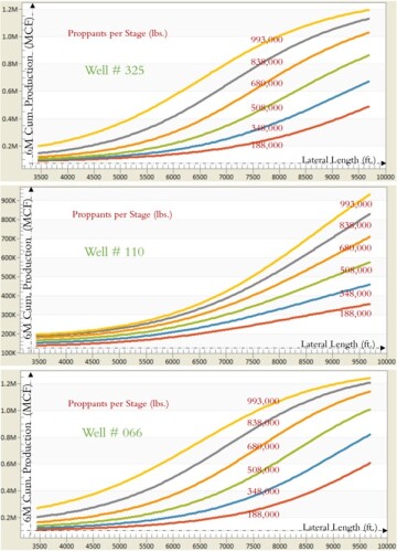
Type curves in Fig. 16 explain that, in this Marcellus Shale asset, 6-month cumulative gas production of the Well #325 can increases from 0.1 million to 1.2 million Mscf as the stimulated lateral length of this well increases from 3,500 to 10,000 ft. This increase in gas production as a function of stimulated lateral length is nonlinear and can change the way it is shown in this figure when the injection of proppant per stage in the completion design of hydraulic fracturing changes from 188,000 to 993,000 lbm as long as all other variables that have been used to build this model remain the same for this specific well.
If the proppant per stage is 188,000 lbm, then gas production can increase from 0.1 million to 0.5 million Mscf as the stimulated lateral length increases from 3,500 to 10,000 ft. If the proppant per stage increases to 680,000 lbm, then gas production can increase from 0.15 million to 1.03 million Mscf as the stimulated lateral length increases from 3,500 to 10,000 ft.
For Well #110 (the middle graph in Fig. 16) the type curves explain that 6-month cumulative gas production can increases from 100,000 to 950,000 Mscf as the stimulated lateral length of this well increases from 3,500 to 10,000 ft. This increase in gas production as a function of stimulated lateral length is nonlinear and can change the way it is shown in this figure when the proppant per stage changed from 188,000 to 993,000 lbm as long as all other variables that have been used to build this model remain the same for this specific well.
If the proppant per stage is 188,000 lbm, then gas production can increase from 100,000 to 350,000 Mscf as the stimulated lateral length increases from 3,500 to 10,000 ft. If the proppant per stage increases to 838,000 lbm, then gas production can increase from 150,000 to 830,000 Mscf as the stimulated lateral length increases from 3,500 to 10,000 ft.
For Well #066 (the bottom graph in Fig. 16) the type curves explain that 6-month cumulative gas production can increases from 0.1 million to 1.22 million Mscf as the stimulated lateral length of this well increases from 3,500 to 10,000 ft. This increase in gas production as a function of stimulated lateral length is nonlinear and can change the way it is shown in this figure when the proppant per stage changed from 188,000 to 993,000 lbm as long as all other variables that have been used to build this model remain the same for this specific well.
If the proppant per stage is 188,000 lbm, then gas production can increase from 0.1 million to 0.6 million Mscf as the stimulated lateral length increases from 3,500 to 10,000 ft. If the proppant per stage injection of the completion design increases to 993,000 lbm, then gas production can increase from 0.25 million to 1.25 million Mscf as the stimulated lateral length increases from 3,500 to 10,000 ft.
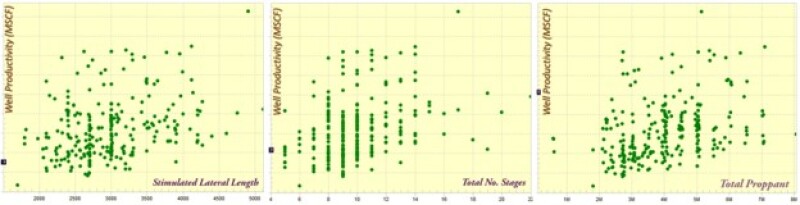
Repeating what was mentioned before, shale analytics (as well as all the applications of AI and machine leaning in petroleum data analytics) does not use any mathematical equations to generate data or to perform any kind of calculations to generate the types of type curves that are shown in Figs. 15 and 16. Actual field measurements that are shown in Fig. 17 were the source of the shale predictive analytics that generate the type curves demonstrated in Figs. 15 and 16. The complexity of the data shown in Fig. 17 clarifies the quality of the XAI that is used in petroleum data analytics.
XAI Model for Conventional Reservoirs—Top-Down Modeling
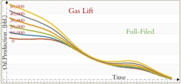
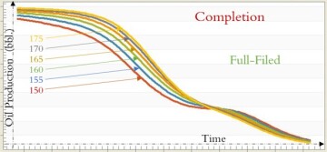
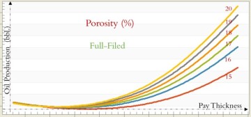
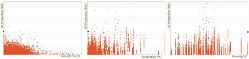
Type curves shown in Figs. 18, 19, and 20 were developed for a mature offshore field in northern Africa using top-down modeling that is a purely data-driven reservoir-modeling technology. These figures explain how and to what degree parameters such as gas lift (Fig. 18), completion (Fig. 19), and porosity (Fig. 20) historically can influence oil production for the entire field.
The well-behaved characteristics of these type curves that were developed using field measurements rather than mathematical equations clearly show how XAI has been used for the development of top-down modeling.
As was mentioned, top-down modeling (AI-based reservoir simulation and modeling) does not use any mathematical equations to generate data or to perform any kind of calculations to generate the type curves that are shown in Figs. 18, 19, and 20. Actual field measurements that are shown in Fig. 21 were the source of the top-down modeling reservoir simulation that generates the type curves demonstrated in Figs. 18, 19, and 20. The complexity of the data shown in Fig. 21 clarifies the quality of the XAI that is used in petroleum data analytics.
Conclusions
Petroleum data analytics is a solid engineering application of AI and machine learning that has the capability of addressing all petroleum-engineering-related problems. Engineering application of AI and machine learning has many differences with the nonengineering application of this technology (e.g., artificial general intelligence). One of the major characteristics of petroleum data analytics is its use XAI. Purely data-driven models that are developed through petroleum data analytics are not black-box models. Petroleum data analytics started to go above and beyond extraction and recognition of correlation from field measurements and started to address causation. While this was done in late 1990s and early 2000, it was not called XAI at that time. Now, especially since 2016, XAI has become an important topic in nonengineering applications of AI and machine learning while it was addressed more than a decade before that time by engineering application of AI and machine learning through petroleum data analytics.
