

Introduction
Petroleum data analytics is a solid engineering application of data science in petroleum-engineering-related problems. The engineering application of data science is defined as the use of artificial intelligence and machine learning to model physical phenomena purely based on facts (e.g., field measurements and data). The main objective of this technology is the complete avoidance of assumptions, simplifications, preconceived notions, and biases.
One of the major characteristics of petroleum data analytics is its incorporation of explainable artificial intelligence (XAI). While using actual field measurements as the main building blocks of modeling physical phenomena, petroleum data analytics incorporates several types of machine-learning algorithms, including artificial neural networks, fuzzy set theory, and evolutionary computing. Predictive models of petroleum data analytics (data-driven predictive models) are not represented through unexplainable black-box behavior. Predictive models of petroleum data analytics are reasonably explainable.
In the early 1990s, when artificial intelligence and machine learning started to be used to solve engineering-related problems, engineers and scientists started asking how this technology achieves its predictive objectives. What recently is being addressed as XAI for the nonengineering application of artificial intelligence and machine learning is not new in the context of engineering application of this technology. The main reason behind the fact that the engineering application of artificial intelligence and machine learning, to a large extent, is quite explainable has to do with the historical problems of the application of traditional statistics in solving engineering-related problems.
While traditional statistics’ main solutions are about identification of correlations in the data, engineers and scientists were always interested in causations that are capable of explaining the correlations. This has always been one of the main problems associated with the use of traditional statistics to solve problems. Many data-driven solutions still are referred to as “black box” solutions. Engineering application of artificial intelligence and machine learning does not generate black-box solutions.
Questions by engineers and scientists gave rise to research and development efforts in the early 2000 and resulted in what today is called XAI. In this article, the history of what is now called XAI is shown through seven technical papers in the oil and gas industry that were published between 2001 to 2010.
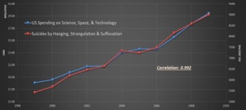
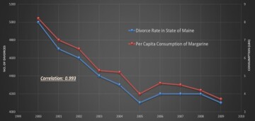
Historically, before the development of artificial intelligence and machine learning, traditional statistics was used to analyze data. The major role of traditional statistics is to specify hypotheses that can fit the collected data. Therefore, the key behind the traditional statistics is correlation, while engineers and scientists have always been interested in causation. It is a well-established fact that correlation does not necessarily determine or represent causation. Figs. 1 and 2 are good examples of how correlation does not have anything to do with causation. These figures demonstrate how data collected for different variables can be correlated while absolutely having nothing to do with one another. Interesting examples of such approaches (correlation vs. causation) are equally true when artificial intelligence and machine learning have been used in the oil and gas industry by those that have no petroleum engineering domain expertise.
Poor applications of artificial intelligence and machine learning in the oil and gas industry (of which I have seen a very large number) are hardly ever exposed. One exposed example of application of artificial intelligence and machine learning in the petroleum industry is when an operating company in the Bakken in North Dakota intended to use artificial-intelligence experts to provide it with data analytics. Based on the collected data, the expert’s concluded that hydrocarbon production from shale wells in the Bakken is controlled by the North Dakota weather. Historically, many major operating companies, as well as the largest service companies in the petroleum industry, have been using artificial-intelligence experts with no domain expertise as their data analytics leadership. Some details about our industry’s approach to artificial intelligence and machine learning have been covered in an SPE Petro Talk.
The objective of this article is to cover and illustrate XAI and demonstrate its initiation as part of petroleum data analytics almost 2 decades ago. Different sections of this article will cover how models that are developed through petroleum data analytics can explain the physics of the models that are generated using purely data-driven artificial-intelligence-based algorithms that do not use any data generated by mathematical equations.
History of XAI in Petroleum Data Analytics
Since 2001, seven SPE papers have been published that include what today is called XAI. These seven SPE papers have a total of 38 figures that use predictive-analytics models to explain how these models can explain the physical phenomena that was modeled purely based on field measurements rather than mathematical equations. To show the historical application of XAI in petroleum data analytics, this article shows figures from these seven SPE technical papers.
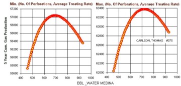
The first technical paper that included the first version of what today is called XAI was an SPE paper (SPE 72385) that was published in 2001. This paper is about the application artificial intelligence and machine learning in modeling hydraulic fractures. Fig. 3 shows a couple of XAI-related figures from this SPE paper. In this paper, the data-driven model that was developed (trained, calibrated, and validated) using artificial neural network to explain the effect of three hydraulic-fracturing-related parameters. These hydraulic-fracturing-related parameters are number of perforations, injection rate, and total amount of water injected. The XAI in this paper explains the effect of these parameters on well productivity (5 years cumulative gas production). Such explanations of the influence of these parameters on well productivity are used to identify well-productivity optimization as a function of the number of perforations, the injection rate, and the total amount of water injected.
Fig. 3, which shows the paper’s original Fig. 7, explains the conditions under which well productivity (5 year cumulative gas production) can reach its maximum value. For this particular well, the 5-year cumulative gas production can reach its maximum value of 57,050 Mscf as long as the number of perforations and the rate of injection are kept at their minimum values (injection rate at 25 bbl/min and eight perforations) and can reach its maximum value of 63,400 Mscf, as long as the number of perforations and the rate of injection are kept at their maximum values (60 bbl/min for injection rate and 26 perforations).
As shown Fig. 3, while these parameters (the number of perforations and the rate of injection) are kept at their minimum value, the highest 5-year cumulative gas production (57,050 Mscf) is achieved at 680 bbl of water. On the other hand, when these values are kept at their maximum, the highest 5-year cumulative gas production (63,400 Mscf) is achieved at approximately 725 bbl of water injected. The conclusion may be that, for this well, the ideal water injection volume is approximately 700 bbl. This SPE paper include two more similar figures showing such explanation for two more wells in the same field.
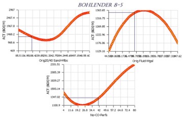
Similar to the paper that was published in 2001, the second technical paper that included XAI was an SPE paper (SPE 77597) that was presented at SPE’s Annual Technical Conference and Exhibition and was published in 2002. This paper also is about the application artificial intelligence and machine learning in modeling refracturing (restimulation) in the DJ Basin in Colorado. Fig. 4 is the explanation of the modification of the well productivity as a function of parameters such as the amount of injected proppant (sand) and fluid as well as the number of perforations. In this figure, the monthly barrel of oil equivalent as well productivity is show for Well Bohlender 8-5 during refracturing.
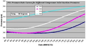
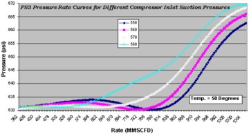
The third technical paper that included XAI was an SPE paper (SPE 77659) that was also published in 2002. This paper covers purely data-driven modeling of BP’s Prudhoe Bay surface facility in Alaska using artificial intelligence and machine learning. This paper includes figures that generate XAI covering separator pressure, temperature, hydrocarbon rates, and compressor inlet suction pressure of eight different three-phase separator facilities. Figs. 5 and 6 show two such figures from this SPE paper.
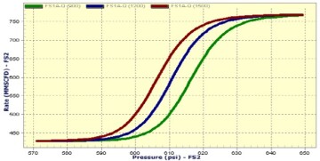
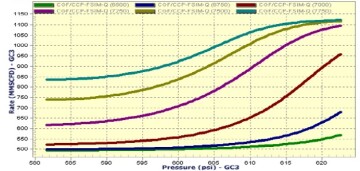
The fourth technical paper that included XAI was an SPE paper (SPE 89033) that was published in 2004 that included more examples of XAI from the Prudhoe Bay’s surface facility’s purely data-driven model. This paper includes seven figures that cover XAI of the Prudhoe Bay’s surface facility. Figs. 7 and 8 show two such figures from this SPE paper.
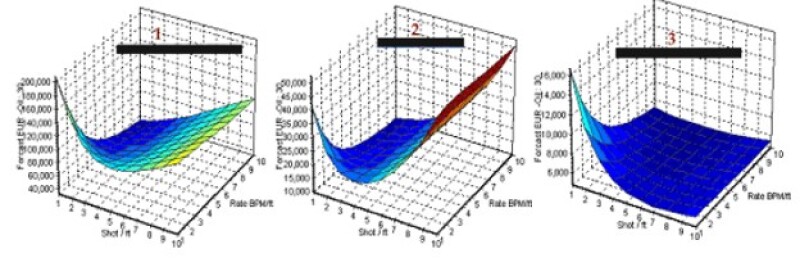
The fifth technical paper that included XAI was an SPE paper (SPE 95942) that was published in 2005. This paper covers XAI of hydraulic fracturing in the Golden Trend field of Oklahoma. This paper includes two figures that show XAI results for the hydraulic fracturing of multiple individual wells in this field.
Fig. 9 explains how shots per foot (x axis) and injection rates [(bbl/min)/ft] (y axis) influence 30-year estimated ultimate recovery for three individual wells. These wells show different types of responses as the number of perforations and average rate of injection per foot of pay thickness changes. The production response is different for each of these wells as the number of perforations and the average injection rates start to increase.
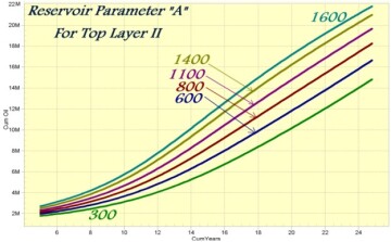
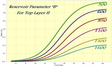
The sixth technical paper that included XAI was an SPE paper (SPE 101474) that was published in 2006. This paper covers XAI of smart proxy modeling of traditional numerical simulation models. Fig. 10 provides type curves of the model that demonstrates the effect of a specific reservoir parameter on oil production, while Fig. 11 provides type curves of the model demonstrating the effect of another specific reservoir parameter on water cut.
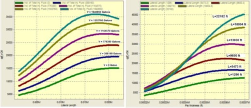
The seventh technical paper that included XAI was an SPE paper (SPE 139032) that was published in 2010. This paper covers completion design characteristics of hydraulic fracturing in the Bakken Shale. The XAI model that is shown in this paper was developed using the IMagine software that is used to develop top-down models. Fig. 12 demonstrates the use of XAI to explain the oil production characteristics as a function of lateral length and injected fracturing fluid (graph on the left) and the oil production characteristics as a function of pay thickness and lateral length (graph on the right).
Watch for Part 2, coming soon.
