
Motivation
Large geological models are needed for modeling the subsurface processes in geothermal, carbon-storage, and hydrocarbon reservoirs. Because of the large spatial extent of subsurface reservoirs and the associated heterogeneity, geomodels are usually very large, containing millions of cells. Large geomodels significantly contribute to the computational cost of history matching, engineering optimization, and forecasting. To reduce this cost, low-dimensional representations need to be extracted from these geomodels. Deep-learning tools, such as autoencoders, can find geologically consistent low-dimensional representations of large field-scale geomodels.
In this work, traditional autoencoders (AE), such as a variational autoencoder (VAE), and advanced autoencoders, such as a vector-quantized variational autoencoder (VQ-VAE) and hierarchical VQ-VAE, referred as VQ-VAE-2, are used to find low-dimensional representation of a geomodel made of 60,000 cells. Structural similarity index metric (SSIM) is used to measure the geological consistency of the newly extracted low-dimensional representations. SSIM arranges from 0 to 1, with higher values indicating better reconstruction.
Deep-Learning Models for Extracting Low-Dimensional Representations
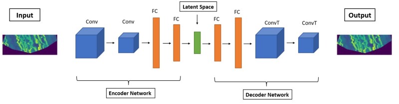
AE. AEs are unsupervised neural networks that can learn the low-dimensional, nonlinear representations of large spatial data (e.g., images). As shown in Fig. 1, they consist of three components—encoder network, decoder network, and latent space (also referred as latent vector, latent code, or bottleneck layer). The encoder maps the input data to a latent vector. The decoder maps the latent vector back to recover the input data. The aim of the AE network is to learn the latent vector, such that the decoder output is as close as possible to the input. The learning requires minimization of a suitable reconstruction loss function, which can be root mean square error, mean squared error, or categorical cross entropy, to name a few.
VAE. Similar to AE, VAE consists of encoder network, latent space, and decoder network. The encoder maps the input data to a multivariate latent distribution instead of a latent vector. The decoder then samples a latent vector from the latent distribution and tries to accurately reconstruct the input data. Unlike AE, the latent space of VAE is regularized using Kullback–Leibler divergence such that similar samples get projected close to one another and dissimilar samples are projected away from one another. Compared with AE, the latent space of a VAE is continuous, centered, and easier to interpolate. Instead of learning a latent space, VAE learns a latent distribution, from which latent vectors are sampled by the decoder for reconstruction of input data. Unlike AE, VAE has generative ability. In other words, the decoder of VAE can be used to generate new samples not contained in the training data set because the VAE latent space is quasicontinuous, centered, and evenly spread without gaps.
VQ-VAE. VAE uses continuous latent space that suffers from posterior collapse when the encoder becomes weaker and the decoder starts ignoring the latent vectors. Posterior collapse leads to extremely blurry reconstruction. Learning a continuous latent space is challenging and is not needed for a variety of tasks, such as sequential decision making. Unlike VAE, VQ-VAE uses a discrete latent space to achieve discrete representation learning, which is suited for sparse image, audio, and video data that can be represented as a combination of discretized information. For example, audio speech can be discretized into combinations of approximately 50 sounds. VQ-VAE has the standard structure of an autoencoder—encoder network, discretized latent space, and decoder network. Discrete latent space prevents the encoder from encoding weak information while providing faster optimization in the presence of sparse data.
The architecture of VQ-VAE is presented in Fig. 2. The discretized latent space is constructed using a codebook containing learnable embedding vectors, which are learned by minimizing the codebook loss. For each input data, the encoder network learns to generate encoder output that is as close as possible to a few selected embedding vectors in the codebook. This assignment of encoder output to certain embedding vectors in the codebook using a nearest neighbor lookup is known as vector quantization (VQ). The learning of the encoder network is guided by commitment loss and reconstruction loss. The decoder network learns to sample a sequence of certain embedding vectors from the codebook to reconstruct the input data. The decoder network learns by minimizing the reconstruction loss. Details of vector quantization can be found in the complete paper.
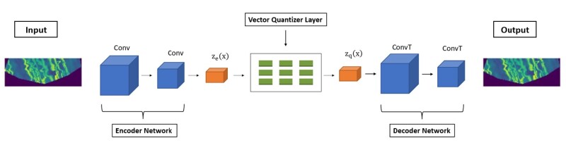
Reconstruction loss is used to tune both the encoder and decoder. The codebook loss is used to keep the embedding vectors close to encoder output (i.e., the embedding vector moves closer to the encoder output). The commitment loss tunes the encoder. It ensures the encoder outputs “commit,” or move closer to the embedding vectors they have been assigned to in the previous iteration. Commitment loss prevents the encoder output from fluctuating too frequently from one code vector to another.
Hierarchical VQ-VAE (VQ-VAE-2). VQ-VAE-2 is similar to VQ-VAE in its working principle. It is a hierarchical organization of VQ-VAE and, thus, consists of two decoders, two encoders, and two VQ layers. The hierarchical structure of VQ-VAE-2 ensures better reconstruction compared with VQ-VAE. The hierarchical multiscale latent maps increase the resolution of reconstruction.
Results and Discussion
Extremely Low-Dimensional Representation of Subsurface Earth. VQ-VAE-2 compresses each layer in the geomodel to generate integer-valued bottom code and top code. Each geomodel has nine layers, and each layer contains 6,912 cells. The top and bottom codes computed using the VQ-VAE-2 are small-sized vectors (Table 1). The top code represents global information, while the bottom code represents details and local information. The top code captures the global structure of spatial variations in the geomodel layer. The bottom code contains the local details and finer structural variations in the geomodel layer. Each component in the code has an integer value ranging from 0 to 1,023. Table 1 presents the integer-valued latent codes. All the colormaps for VQ-VAE-2 range from 0 (black) to 1,023 (yellow) in the viridis colormap because VQ-VAE-2 uses a codebook size of 1,024.
The top row of Table 1 presents four geomodel layers of varying geological complexity, arranged from simple on the left to complex on the right. The geomodel show the porosity distribution across a 15×5 km region. The second row of Table 1 shows the low-dimensional representations (i.e., latent codes) obtained using VQ-VAE at a compression ratio of 155. The last three rows of Table 1 present the low-dimensional representations obtained using VQ-VAE-2 at compression ratios of 167, 417, and 667. VQ-VAE-2 at compression ratio of 167 generates 8-dimensional top code and 32-dimensional bottom code, while, at compression of 417, VQ-VAE-2 generates 8-dimensional top code and 8-dimensional bottom code. VQ-VAE-2 at compression ratio of 667 is compressing the 6,912 cells to 2-dimensional top and 8-dimensional bottom codes. At a compression ratio of 667, the top codes of simpler layers are different from those of complex layers. The extremely low-dimensional representations obtained using VQ-VAE and VQ-VAE2 vary with the change in the geological complexity of the geomodel layers.
More details and visualizations of the low-dimensional representations can be found in the complete paper.

Compression and Reconstruction Performances of the Optimized Deep-Learning Models. The best results, in terms of compression ratio, for the chosen architecture for each model are presented in Table 2. The results are shown for geomodels with increasing complexity (number of channels in the reservoir). The geomodel layers show the spatial variation of porosity across a 15×5 km region. There are 2,000 geomodels in the data set. 20% of the geomodels were used as test. Each geomodel contains nine layers. Each layer of geomodel contains 144×48 cells. A good reconstruction in terms of SSIM at a high compression ratio ensures geological consistency and reliability of the low-dimensional representations extracted from the large geomodels.
Traditional singular value decomposition (SVD) with 700 singular values provides an approximate reduction factor (compression ratio) of 10 that can be used to reconstruct the original geomodel at a structural similarity index metric (SSIM) of 0.9. AE, VAE, VQ-VAE, and VQ-VAE2 performed significantly better than the well-established SVD approach. SSIM arranges from 0 to 1, with higher values indicating better reconstruction. SVD at a compression ratio of 10 achieves SSIM of approximately 0.91 when reconstructing the four layers of varying geological complexities. An increase in compression ratio of SVD to 50 drastically decreases the SSIM of reconstruction for the first three layers to 0.77. For the most complex layers, SVD, VAE, and AE are not able to reconstruct the complex channels. Table 2 shows VQ-VAE is better compared with SVD, VAE, and AE. For all four layers, VQ-VAE-2 at a compression ratio of 167 performs better than VQ-VAE at a compression ratio of 155. VQ-VAE reconstructions are blurry compared with those of VQ-VAE-2. An increase in compression ratio of VQ-VAE-2 from 167 to 417 does not drastically change the reconstructions, which are still better than VQ-VAE reconstruction at a compression ratio of 155. Reconstruction performance of VQ-VAE-2 at compression ratios of 417 and 667 are relatively the same. Overall, this study clearly shows the amazing performance of VQ-VAE-2 in massively compressing large geomodels to obtain extremely low-dimensional representations.
More details and visualizations of the reconstructions using the low-dimensional representations can be found in the complete paper.