The objective of the complete paper is to accurately determine horizontal-shale-well estimated ultimate recovery (EUR) for an area integrating geology, machine learning, pattern recognition, and statistical analysis by use of various parameters of nearby producing horizontal shale wells as inputs. The work uses local geological information followed by execution of machine learning to identify critical well parameters that lead to better production. Then, a pattern-recognition step is performed while making sure the number of wells in each category is statistically significant. The conclusions are verified using available literature on correlation between well production and various well parameters. Along with the prescribed big-data mining methodology, the most important conclusion from this study is that for the optimal evaluation of shale assets, it is critical to tie in the controllable well parameters to well production. Once this relationship is established, the type-curve determination and the EUR estimation can be performed more accurately.
Methodology
This work focuses on determining the EUR for different local regions with several nearby horizontal shale wells. The objective is to select only those wells that have optimized completions for each bench and potentially develop separate type-curves for each bench. The first step is determining in advance which well parameters may be important. This involved consideration of other researchers’ work and the general direction in which the industry is headed (more proppant, longer laterals, and landing depths). The second step is identifying pre-existing correlations between well parameters—for instance, ppg and fluid/ft should ideally be correlated. These pre-existing correlations deteriorate the quality of identified relationships between the performance and variables. The ranges of selected variables were evaluated for quality-control purposes. If there were obvious outliers that could have been a result of an error in reporting, they were removed. Because of the unavailability of petrophysical-properties maps at the time of initial assessment of the assets, they were not included in this data analysis. However, once the identified pattern revealed a relationship between better production and landing depths, the local specialized shale logs were evaluated to determine the difference in petrophysical properties among different benches.
The author believes that, for the most robust evaluation, a twofold methodology should be applied to any asset-evaluation exercise, in which the general profile of the asset is considered before a well-by-well analysis is performed.
Case Study
The complete paper discusses a case in the Permian basin. The Wolfcamp formation (primary target) is approximately 1,000 ft thick in this area and has multiple landings (benches). Wolfcamp top depths were used in creating a contour overlying the map. Only those wells lying on similar Wolfcamp structures (indicated by contours) had been selected for analyzing a shale asset for acquisition and divestiture potential. The area to be analyzed was small and confined to a similar depositional environment with respect to each bench (landing depth).
The asset looked uneconomic if the type-curve (EUR) was obtained by averaging all the horizontal Wolfcamp wells on production. The challenge for the technical team was to demonstrate to management and potential investors that the area had an upside potential even at depressed oil prices. There were almost 250 wells in this study. Statistically, a number more than 30 is reasonable from which to derive patterns, considering that the number of well variables used in multivariate analysis is relatively smaller.
The performance parameter selected for the analysis is 6-month cumulative production normalized to a lateral length of 10,500 ft. It is referred to as Y in the complete paper at several instances. A multilinear regression was performed assuming linear dependence of Y on the individual well parameters.
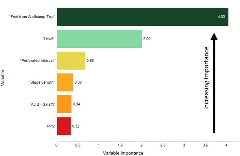
Fig. 1 shows the resulting tornado plot. The plot ranks the variables in order of their importance in influencing Y. It is evident that the deeper landings relative to Wolfcamp top and higher lbm/ft (proppant loading) were most concurrent with enhanced well production. The p-value associated with each of these variables, which was less than or equal to 0.05, was considered to be a threshold value for relevance in correlation between Y and well variables. If one assumes the criticial value to be 0.05, this model demonstrated that only the landing depth (higher values) and proppant loading (higher values) were stastically significant regarding their concurrency with better well performance.

The null hypothesis H0 (no dependence of Y on a variable) cannot be denied for variables with p-values greater than 0.05. The t-value, which is indicative of how many standard errors is the estimate away from “0,” determines the variable importance. It should be noted that even when the p-value is greater than 0.05 but relatively small compared with the other variables, it implies a moderate correlation between the well variable and the well-production metric.
It is important to understand that, in truth, no model is perfect. The underlying assumptions (linear dependence and nearly normal distribution) can easily be challenged. The diagnostic plots can further illuminate the imperfections of the relationships described previously. On the contrary, the reservoir engineer uses these tools only to identify patterns to keep in mind for further analysis and field development. The key decisions are made by use of other resources as well.
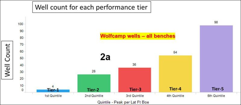
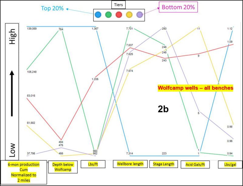
The next step was to visually inspect the multivariate plot and identify any patterns that may be evident. It is important to show the histogram for the wells falling in each performance tier (Fig. 2a). There are more wells in the lower tiers than in the upper tiers. In other words, there are more underperforming wells than overperforming wells. This can easily dissuade any team from any potential acquisition in this area. However, it is important to consider the relatonships between well performance and completion parameters identified, as previously discussed. Fig. 2b is a multivariate plot. The first parameter on the X-axis is the cumulative 6-month production and the others are well variables. The labels at each node are the respective values for each variable. Comparing Tier 2 (26 wells) with Tier 5 (98 wells) reveals that some of the patterns identified by the machine-learning algortihms are quite evident. Wells in deeper landing depths and/or higher proppant loading tend ot have better production. It is interesting to note that the depth targeted by Tier 1 and 2 wells was approximately 300 ft deeper than Tier 3, 4, and 5 wells. Tier 1 and 2 wells target the same deeper Wolfcamp zones with divergent proppant usage and divergent production results (a difference of 25,000 BOE in 6-month cumulative production normalized to a 10,500-ft lateral). The same applies to Tier 3 and 5 wells targeting shallower Wolfcamp benches. Tier 3 and 5 wells have similar wellbore and stage lengths.


The strong correlation between deeper landing depths and better well production necessitated the need to understand the rock/pressure changes along the depth of the Wolfcamp formation. The Wolfcamp is almost 1,000 ft thick in this area. The formation is normally pressured (less than 0.5 psi/ft). The operators active in the area have delineated the formation into three benches, A, B, and C. For the purposes of the paper, the benches were addressed as shallow, middle, and deeper. This delineation might have emanated from the various flooding surfaces in the Wolfcampian period.
Discussion of Results
This study demonstrates the use of big-data mining techniques (machine learning, pattern recognition, and applied statistics) in determing the type-curves (and the resulting EUR) for an asset being evaluated for acquisition. Using the available well data for wells landed in the 1,000-ft-thick Wolfcamp section, the prescribed methodology demonstrated concurrency of better well results with choice of landing depth and proppant loading. This necessitated the need to analyze wells in different Wolfcamp benches individually. The complete paper establishes that in different benches, different controllable completion variables were concurrent with better well production. This study illuminated the hidden upside value in a shale asset that appeared to be subeconomic. Extensive geological study along with specialized shale-log cross-sections can further assist a team in making more-informed decisions
It must be remembered that applied statistics and machine learning can help guess future performance if the data points stay in realm of the several variable ranges in the study. For example, if the industry is moving toward 2,500 lbs/ft, the described study cannot predict the performance of such wells, because there is only one well in the study that used 3,000 lbs/ft. The same applies to other variables. The models generated here cannot predict well performance in another county of the Permian basin. The author does not wish to convey the idea that improved completions design beyond the realm of the existing wells will not assist in better production. However, when it comes to investment decisions, the existing wells with reasonable completions in the potential acquisition area need to be demonstrated as economic.
The author was with Texas Standard Oil LLC when the article was written. He is now a Petroleum Engineering Consultant with Bruin E&P Operating.

