When fluids are injected into formations at high rates, underground rocks break and vibrate, creating extremely low-frequency energy, like a giant subwoofer. Subsurface infrasound signals can be generated during fluid-driven volumetric processes in different geological settings such as volcanoes, geysers, and oceanic magma. This article shares a data-driven work flow used to locate and monitor the infrasound and near-infrasound sources (2–80 Hz) in the stimulated reservoir volume (SRV).
To that end, the work flow analyzes the low-frequency signals in the hydrophone measurements acquired during a mesoscale (~10 m) hydraulic-fracturing field experiment at a depth of 1.5 km. This approach revealed sections of rock deformation in the SRV that were not visible using traditional microseismic imaging. Combining these infrasound signals with microseismicity signals allows for better characterization and monitoring of the SRV.
The newly developed data-driven work flow for a novel infrasound imaging will be valuable for locating and monitoring subsurface fluid pathways, tremendously improving geothermal and hydrocarbon resource development.
Site for the Hydraulic-Fracturing Field Experiment
This article presents a new data-driven analysis to locate the low-frequency seismic sources (2–80 Hz), referred to as near-infrasound or infrasound sources. The study further investigates the relationship of the infrasound sources to microseismicity and modeled natural fractures. More detail of the study is available in Chakravarty et al. (2022).
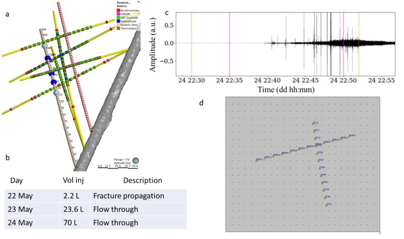
The study uses hydrophone data generated by the EGS Collab Project, a unique mesoscale, densely instrumented test site located in Leads, South Dakota, and funded by the US Department of Energy. The EGS Collab Experiment 1 is a mesoscale (~10 m) hydraulic-fracturing field experiment situated at the Homestake Gold Mine in Leads, South Dakota, at a depth of 1.5 km. The aim of the intermediate-scale field study is detailed characterization of hydraulic fracturing through dense geophysical instrumentation of the stimulated rock volume (Kneafsey et al. 2020; Chakravarty and Misra 2022). Fig. 1 describes the intermediate-scale field study in more details.
Infrasound Energy Generated During the Hydraulic-Fracture Field Experiment
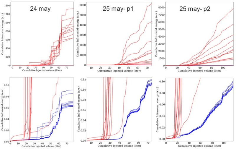
Fig. 2 shows the energy detected in the infrasound and near-infrasound frequency band (8–20 Hz) during the hydraulic stimulation at the intermediate-scale field study. In Fig. 2, the infrasound energy is correlated to the injected fluid volume. Two orthogonal hydrophone strings, E1-OT and E1-PDB, each consisting of 12 hydrophones, recorded the infrasound and infrasound emission during fluid injections. As the hydrophones on the well E1-OT are closer to the fluid-driven deformation, the incident infrasound signal intensity is greater on the E1-OT hydrophones. The infrasound energy measured by E1-OT (Fig. 2, red) hydrophones is five orders of magnitude greater than the distant string E1-PDB (Fig. 2, blue). Note that, as the experiment proceeds, the gradient of cumulative infrasound energy for both the hydrophone strings becomes progressively smoother. Impulsive energy release indicative of stick/slip type of fracture propagation is dominant on 24 May, wherein the energy release is in discrete bursts, resulting in strong ridges in the cumulative energy curves from all sensors. Fluid flow through fracture conduits generates long-period infrasound tremors, indicative of long-duration energy release. This transition indicates a regime change from fluid-driven fracture propagation to fluid flow through fractured conduits.
Data-Driven Analysis To Locate Infrasound and Near-Infrasound Sources
Because of the emergent nature of the signals, we used a grid search approach based on cross-correlation, which has been commonly used for identifying sources of tremors on local and regional scales (Wech and Creager 2008). The algorithm requires the input of a hydrophone signal, a grid (Fig. 1d), and a velocity model. We set the grid dimensions to match the hydrophone network and extended it by 30% in both directions, while using an isotropic velocity of 5.5 km/s for the compressional wave. The rolling window location algorithm works by cross-correlating pairwise signals from every station at each window and measuring their similarity as a function of signal displacement. The time lag calculated from the correlogram is compared with the calculated theoretical time lag between station pairs based on the input velocity model. By minimizing the difference between the modeled and observed objective functions, the grid node with the minimum misfit is identified as the source location.
Given a suitable isotropic velocity model, the key parameters determining the source locations of the algorithm are the window length and window overlap. Determining the signal duration of emergent signals is nontrivial because of uncertainty in detecting first arrivals. Application of short-term average/long-term average (STA/LTA) methods usually lead to overestimating the pulse duration. To get an estimate of the pulse duration, we applied the STA/LTA filter to a sample of hydrophone data from well E1-OT and then corrected for the overestimation. An average value of 1 second was obtained as the average pulse duration of the infrasound signals. With this information, a window length of 1 second and window overlap of 0.5 second is chosen for subsequent analysis.
Post-Processing To Refine the Infrasound/Near-Infrasound Source Locations
The data-driven, grid search algorithm is prone to false positives. Hence, a series of post-processing filters is applied to determine reliable low-frequency source locations.
- The first filter sets an upper bound of 0.95 and a lower bound of 0.6 on the normalized cross-correlation coefficients of the windows. Windows outside these bounds are discarded because they may contain correlated noise or uncorrelated signal.
- The second filter uses the relative power of the hydrophone array computed throughout the experiments to discard located timestamps with normalized beam power below the noise floor. A threshold value of relative power (0.3) is used to differentiate located and nonlocated timestamps.
- The third filter uses bootstrapping to perform 20 iterations for the cross-correlation-based locations. In each iteration, 5% of the cross-correlograms are removed randomly and the resulting scatter is considered a measure of location uncertainty. The data points with the highest 10% of scatter values are discarded.
- The last filter uses the misfits obtained in the grid search algorithm to discard data showing the highest misfit values. 50% of the data with the highest misfit values are removed. Despite losing half the data, the spatial coverage of the source locations shows little change, demonstrating the effectiveness of the misfit filter.
Spatiotemporal Evolution of Infrasound/Near-Infrasound Sources Compared With Microseismic Sources
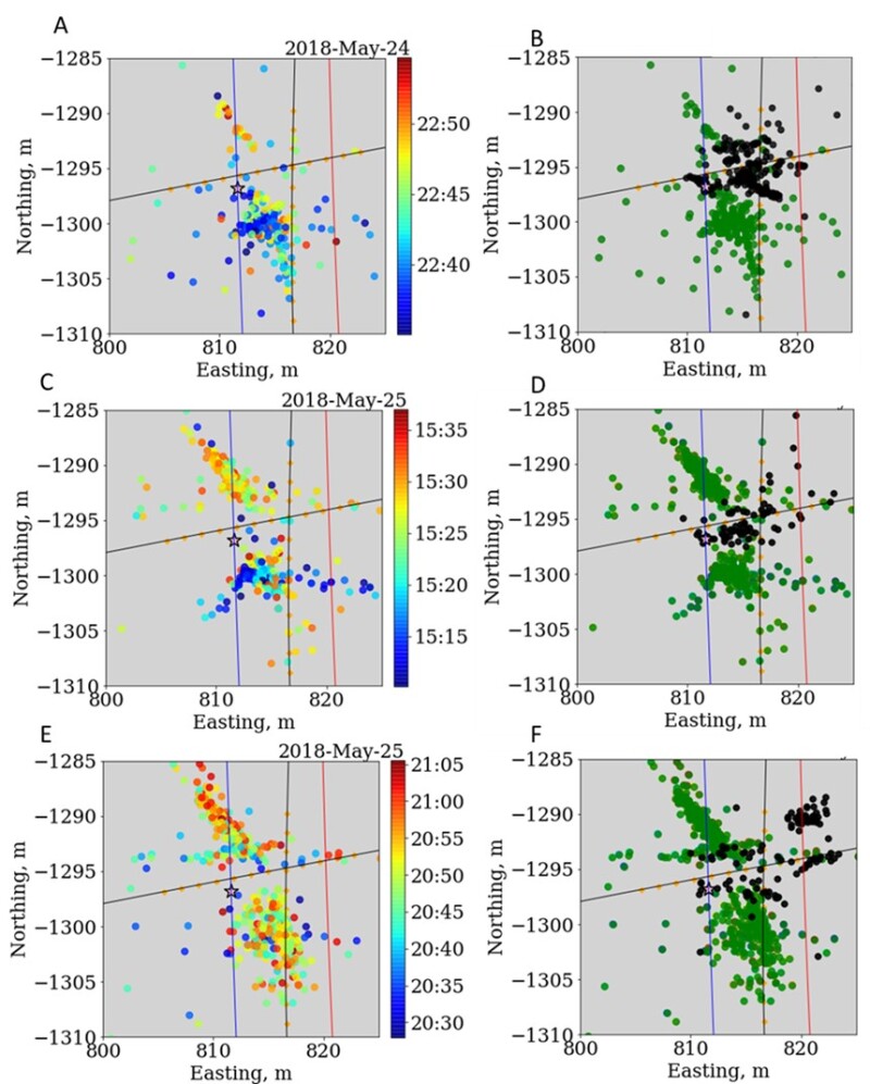
Fig. 3 illustrates the evolution of the newly identified infrasound/near-infrasound source locations over time. During the early time on May 24, the sources spread out perpendicular to the injection well (Fig. 3a). Beyond 2245 hours UTC, the sources become concentrated along a lineament that is subparallel to the injection well, and subsequent events follow the same direction but migrate northward from the injection point. In Part 1 of May 25 (Fig. 3c), the sources have a less diffuse distribution than before, with early-time sources along an east/west trend south of the injection point and later events forming a relatively sparse line trend to the north of the injection point. Two subparallel lineaments in an east/west direction are also observed. At the beginning of injection in Part 2 of May 25 (Fig. 3e), the infrasound sources fall on the previously described two lineaments on either side of the injection point, being subperpendicular to the injection well, and later events align subparallel to the injection well.
The joint analysis of infrasound/near-infrasound sources (green) and microseismic sources (black), as shown in Figs. 3b, d, and f, encapsulates frequencies on the observable bounds of acquisition instrumentation (2 Hz to 15000 Hz). As a result, both high- and low-frequency fracturing phenomena driven by fluid injection are captured. The joint data reflects fluid-injection-induced subsurface deformation that lies on a continuum, with one end representing high-frequency, small-scale shear slippage on fractures and the other end representing low-frequency, large-scale void volume dilation or contraction. This leads to the conclusion that microseismicity and infrasound signals contain complementary information about rock deformation because of fluid injection, and their joint analysis renders a more complete picture of the stimulated fractures in subsurface.
Proposed Mechanisms Governing Infrasound/Near-Infrasound Sources
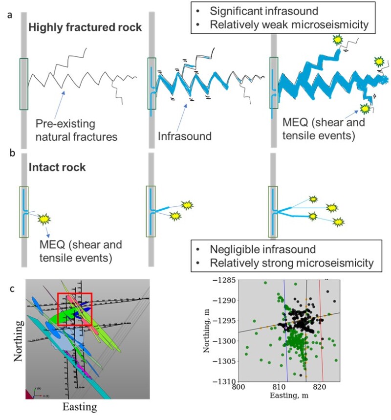
Through joint analysis of high- and low-frequency signals, more information can be obtained about fractures compared with using only one method. Fluid injection into fractured rock can cause cracks to expand or contract, creating mechanical waves that generate both high-frequency shear motion and low-frequency P-waves. This is illustrated in Fig. 4, which shows the orientation and distribution of natural fractures in a discrete fracture network. The presence of microseismicity indicates fluid interactions mobilizing critically stressed cracks, while infrasound activity suggests pressurized natural fractures that generate low-frequency compressional motion. The highly fractured rock leads to significant infrasound measurement and relatively low microseismic measurement, while the intact rock environment results in negligible low-frequency seismic and relatively greater occurrence of high-frequency microseismic. Moreover, the attenuation of high frequency signals is far less in intact rock compared with fractured rock, resulting in more high-frequency signals being generated and more easily measured by sensors.
Conclusions
A total of 322, 818, and 1,117 infrasound source locations were obtained for the 3 days of stimulations. Impulsive energy release at earlier stages corresponded to fracture propagation, while a smoother release at later stages of stimulation corresponds to tremor-like motions generated from fluid flow in conduits. Infrasound signals of usable signal-to-noise ratio are produced only at relatively high fluid-injection rates. The infrasound is emergent signal, so first arrival picking from threshold-based methods is rendered inaccurate. Therefore, a data-driven cross-correlation-based grid search was applied to locate the infrasound source locations. Four filtering steps were designed and applied to improve the source locations.
Acknowledgements
This material is based on work supported by the US Department of Energy, Office of Science, Office of Basic Energy Sciences, Chemical Sciences Geosciences, and Biosciences Division, under Award Number DE-SC0020675 and the Texas A&M TRIAD funding. The authors acknowledge the efforts of the EGS Collab team for conceptualizing and executing the experiments and hosting the open-source data. The authors are grateful to Texas A&M High Performance Research Computing staff members for their support.
References
Chakravarty, A., and Misra, S. 2022. Unsupervised Learning From Three-Component Accelerometer Data To Monitor the Spatiotemporal Evolution of Mesoscale Hydraulic Fractures. International Journal of Rock Mechanics and Mining Sciences. https://doi.org/10.1016/j.ijrmms.2022.105046.
Chakravarty, A. et al. 2022. Hydraulic Fracturing-Driven Infrasound Signals—a New Class of Signal for Subsurface Engineering. https://doi.org/10.1002/essoar.10512584.1.
Kneafsey, T. J., et al. 2020. The EGS Collab Project: Learnings from Experiment 1. https://www.osti.gov/biblio/1766466.
Wech, A.G., and Creager, K.C. 2008. Automated Detection and Location of Cascadia TTremor. Geophysical Research Letters. https://doi.org/10.1029/2008GL035458.