Devon Energy may have unlocked why hydraulic fractures in some tight-rock plays grow faster than others. This appears to be strongly linked to the well-density potential of these plays.
The operator is also working on a new way to measure how fractures squeeze steel pipe, which, in turn, might result in more-efficient completion designs.
SM Energy recently studied the interactions between hydraulic fractures and faults in one of its tight-rock projects in Texas. When a fault slipped, the Denver-based producer had seen production slip too.
Now, armed with enough data, SM Energy has adopted new completion designs that avoid overpressurizing the faults found all over the target formation.
Shell’s search for light-tight oil in the Permian Basin ended about a year ago but what the company learned there will live on in its other unconventional projects. Not least of those learnings involves how to best deploy diagnostic technologies to answer big questions about the way fractures behave—no matter the formation.
These glimpses into how each unconventional operator is relying on fracture diagnostics were shared at a recent technical conference organized by Calgary-based SAGA Wisdom which offers training for engineers on reservoir analysis. Here is more on the lessons they shared with the industry at the conference held this year in Fort Worth, Texas.
Pick the Right Tools
Som Mondal, an engineer with Shell’s shale business unit, joked that when he agreed to speak at the conference about the company’s diagnostics journey in the Permian, it still owned assets there. The London-based supermajor exited the largest US onshore play in a $9.5-billion sale to ConocoPhillips that closed in December 2021.
But while it has moved on from the Permian, Shell still operates unconventional assets in Argentina’s Vaca Muerta and the Montney Shale in Alberta. It is in those places where the company’s years of integrated diagnostics research in the Permian will be carried forward.
Mondal shared how that work shaped the way he now views the different diagnostics technologies and where they complement each other. On this, he subscribes to two overarching philosophies.
“One, we need to aim for consilience—which is when different, independent approaches converge toward the same solution,” said Mondal. “And second, we need to weigh the different diagnostics so that we can combine them based on our confidence in them and the scope of its measurement.”
When it comes to putting this into practice, at Shell the work begins with trying to match the technologies to one of these three questions.
- How did my perforations take in fluid and what was the distribution of this intake? The answer relies on fiber optics to measure acoustics, temperature, and strain.
- What is the geometry of my newly created fracture system? Here too, fiber optics provide big insights, but other gaps can be filled in by microseismic, sealed wellbore pressure monitoring (SWPM), and bottomhole pressure gauges.
- What portion of that new fracture space is effectively producing oil and gas into my wellbore? For this question, bottomhole gauges are useful once again, and to an extent so is geochemistry. Well-interference testing (e.g., the Chow Pressure Group method) and/or observation wells are also critical tools.
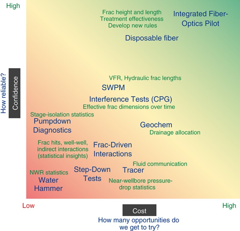
Mondal showed a matrix he created that compares different diagnostics with “reliability” representing one axis and “cost” representing another. More reliable means more confidence in the data. More expensive means you get fewer opportunities in the budget to use the technology.
To the top and right of this matrix, which translates to very reliable but also very expensive, are the integrated fiber-optic projects like those used in the well-known Hydraulic Fracturing Test Site (HFTS) I & II projects.
Notably, through those joint industry projects and its own independent work Shell has been on the leading edge of fiber-optic interpretation for years. Most recently, the operator helped pioneer the use of the technology for strain measurements which can provide a rich picture of whether fractures grow out of each perforation cluster and how they close over time.
However, multiple fiber-optic deployments to measure strain along with temperature and acoustic signals on a single well pad can run up a seven-figure bill quickly. Thus, such efforts tend to represent a once-off for a field‑development project.
At the bottom of Mondal’s diagnostic matrix are tests that can be run on almost every stage but that don’t provide nearly as much resolution as fiber. These include pumpdown diagnostics to test stage‑to-stage isolation along with stepdown tests that help quantify fracture distribution from perforation clusters. To gain valuable insights from these tests Mondal said hundreds may be needed from a given field.
In the middle of the spectrum is the Devon-developed diagnostic SWPM which Mondal said is likely to be needed “tens of times” to help understand fracture geometry in a given field.
A bit lower on the reliability scale for Mondal is geochemistry which in the shale business is most often used to help operators understand which benches are contributing to production and in what proportion.
“I like geochemistry,” said Mondal, “but it’s only as good as the quality of your baseline samples.” Those samples have to be collected and categorized during the drilling phase which is sometimes a difficult process.
Mondal cited geochemistry results from HFTS-II that failed to identify production from zones that were known to be contributing because of more-reliable downhole pressure gauges that directly measure reservoir depletion over time.
Noticeably, the matrix does not include microseismic. That’s not because Shell is not a user of the technology.
Mondal said it is because he considers microseismic to be most valuable when coupled with other complementary technologies in a big diagnostics project, like HFTS I & II. “Used just by itself, it can sometimes be misleading,” he related.
Learn How Faults Work
In early 2021, SM Energy decided to double its efforts on subsurface diagnostics in a patch of tight rock it operates in south Texas called the Austin Chalk. It needed answers on how hydraulic‑fracturing designs were being impacted by the target layer’s abundance of rather sensitive faults.
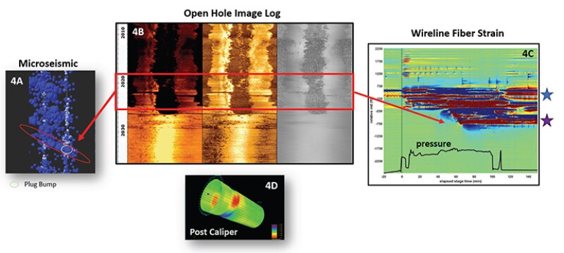
That called for a suite of diagnostic technologies that could each offer a piece of the big puzzle:
- Openhole logging during drilling to confirm fault intersection.
- Perforation-erosion imaging for cluster efficiency.
- SWPM to confirm fracture interactions on offset wells.
- Multiarm caliper to run in offset wells for casing-deformation measurements.
- Permanent fiber optics for temperature sensing (i.e., fluid “warmbacks”).
- Temporary fiber installations for acoustic sensing and microseismic data.
For Erich Kerr, the integrated diagnostics project was illuminating.
The engineering supervisor of reservoir characterization for SM Energy presented the conference with a microseismic dataset showing how the pumping of a fracture stage near the toe-side of the well could cause a fault to move in the heelward direction.
“These faults are activating really early. Sometimes they happen immediately. Sometimes they happen really high. Sometimes they happen thousands of feet ahead” of the stage that is being fractured, Kerr said.
And sometimes, a fault may activate when nothing should be happening at all. Kerr recalled a “bizarre” case where pressure pumping had stopped and pressure within the well was starting to decay. “Then about 30 minutes into that, this weird response started to show up,” he said.
It turned out that response was a fault activating some 500 ft away from the stimulated stage. Modeling work done later with Texas A&M University suggested that the high pressure from the stimulation job was holding the fault closed, but “once we stopped [pumping], it relaxed and the fluid went through the fault,” said Kerr.
Activating a fault in this geology might mean unleashing a torrent of the ancient salt water that sits behind many of them. It’s hard to know this has happened until a new well is popped and excessively high water cuts are recorded.
An opposite issue of sorts can happen too. When some faults slip, the stimulation fluids move through what is a thief zone but not most of the proppant sand. What’s left around the fault is a pack of “dehydrated slurry” that means farther afield regions of the reservoir will not be propped open.
Yet another problem, and one that is more commonly reported by North American operators, is casing deformation. When an immense block of rock suddenly jolts, it can compact or oval a well’s steel casing. This deformation may either require a well intervention or it could totally prevent an impacted stage from being completed.
Kerr noted that SM Energy had seen all three of these fault-driven issues and their impacts on production to varying degrees. “What we think is going on is that we’ve got these faults, sometimes at a high angle, and when we raise backpressure, it counteracts the normal force against the fault and it slips,” he explained.
Whatever design the operator dials up today, it must avoid raising the rock’s pore pressure too much. This is something it does in both the design phase and in real time during the execution of a stimulation.
Overall, after collecting all the subsurface data and using them to calibrate its models and simulations, SM Energy found itself reconsidering nearly every major design criterion for the field. Kerr said changes ran the gamut of well spacing, landing-depth staggering, stimulation sequencing, injection rates, and perforation cluster spacing.
After months of trial and error to test different schemes, Kerr reported that many of the once unpredictable outcomes have been essentially “reversed.” More aspects of the study are covered in a paper Kerr coauthored, SPE 209140, and presented earlier this year.
Stopping “Baseball-Sized” Perf Erosion
As part of its diagnostics project, SM Energy also wanted to focus on achieving better cluster efficiency since it not only relates to fault activation but also overall productivity. Poor efficiency tends to mean overly long fractures were created in a small number of clusters
In one test, SM Energy used a “pretty aggressive geometric design” that Kerr said most shale producers have likely used at one point or another.
“What we found is that on many of the stages where we did this, the stress shadow was way too high and so the toe-side clusters couldn’t even open,” he shared. This was confirmed not only by fiber and microseismic but by also by downhole imaging used to measure perforation erosion.
“On that particular design, sometimes we would have 100 to 150 ft [of wellbore] that was not stimulated, and what that means is that all of that fluid is going into your other clusters,” said Kerr. He added that the dominate clusters were easy to spot since some of them had “baseball-sized erosion.”
Such dramatic erosion can carry the effect of doubling the desired injection rate, which also increases the pressure inside the fracture. In turn, this drives the risk of a “runaway” fracture that exceeds its designed length and/or it could lead to a breakthrough to a previous stage’s already-opened fractures.
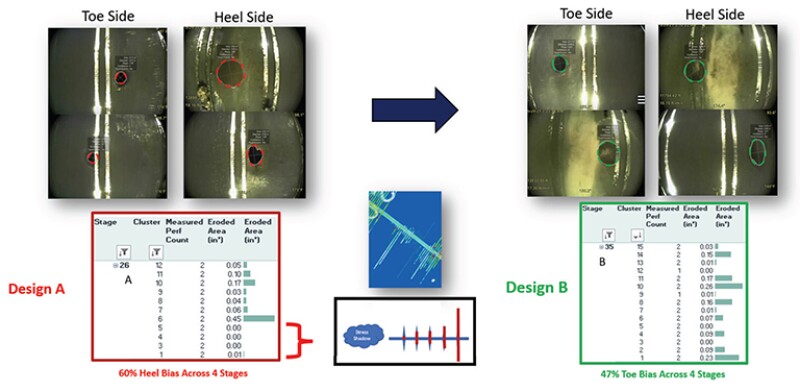
As SM Energy diagnosed the problem, it made changes, particularly to its cluster design and injection rates which resulted in a more-even distribution along the perforations. Kerr said the new design performed especially well in the previously troublesome toe-side clusters.
“All of this came together and the wells were about 5% cheaper,” to complete, he said, adding that the new design took less time to complete and was also producing more oil with less pressure drawdown.
The operator was able to confirm its success using SWPM which enables engineers to compare the number of fracture arrivals vs. the number of clusters. The closer those numbers are, the better.
However, Kerr emphasized that no single technology used in the study delivered all the data needed to know which corrective measures to adopt. “You have to combine these diagnostics together to get a full picture,” he said.
Fracs Grow Fastest in Low-Density Plays
SWPM was but one of the technologies used in SM Energy’s study, but it stands apart as the only one developed by another operator, Devon. In fact, SM Energy collaborated closely with Devon on its use of SWPM in the fault-interaction study.
It works by using a pressure gauge on a sealed, unperforated wellbore that is filled with water. As a fracture approaches from an offset well stimulation and then intersects with the sealed wellbore, a small pressure inflection as low as 1 psi is recorded. That’s all that is needed to know a fracture interaction took place.
This technique has been used by dozens of operators to document fracture interactions in more than 14,000 stages since 2018. Brendan Elliott, a senior staff completion engineer for Devon, shared how the Oklahoma City-based company’s extensive cataloging of its own fracture interactions led it to start developing a number of different applications for SWPM.
But at a minimum, SWPM can be used to determine the growth rate of a hydraulic fracture and the volume of pumped fluids it took to occur—otherwise known as the volume-to-first-response (VFR).
“Looking at well spacing in conjunction with this observation on growth rate gives us early insights into what the appropriate well spacing from basin to basin might be just based on the length of the fractures created generally,” explained Elliott.
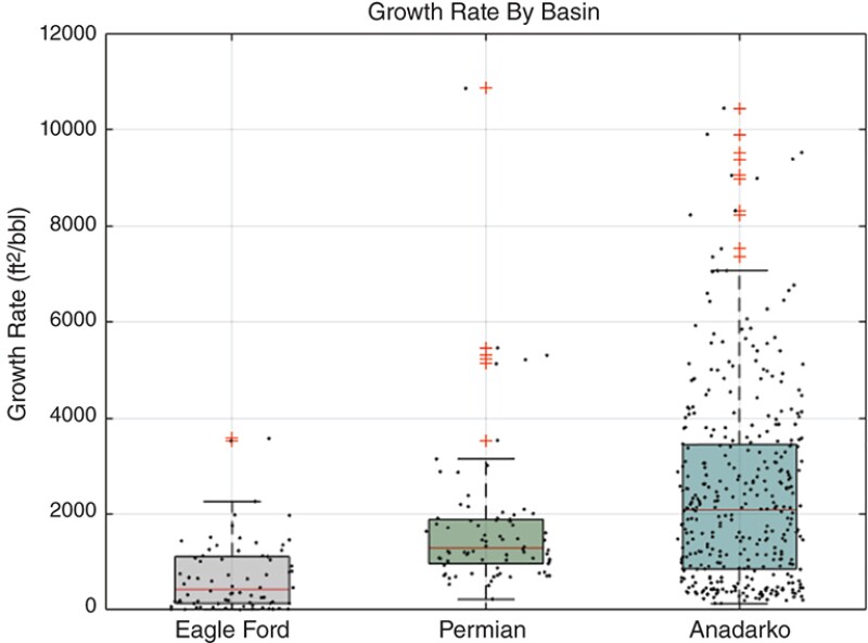
He was showing the result of a dataset inclusive of nearly 1,600 stages from offset wells across the various tight plays Devon operates. Some of the plays exhibit average hydraulic-fracture growth rates that are double or triple that of others.
Where Devon has seen growth rates are highest, and VFRs are generally lowest, is in the Meramec and Turner formations. The former is part of the wider Anadarko Basin in Oklahoma while the latter makes up one of the layers of the Powder River Basin in Wyoming. As a result of these rapidly growing fractures, Elliott said in the Turner formation most operators are drilling one, two, or at most, three wells per section.
Meanwhile average fracture growth in the Bakken Formation in North Dakota is considerably slower. Even less-severe growth rates are observed in the Permian’s prolific Wolfcamp target and in the Eagle Ford Shale.
“What that tells you is in the Anadarko, we can generate much larger fracture geometries per barrel injected than if it was in the Eagle Ford, and that can have all kinds of implications on well spacing and capital efficiency,” said Elliott.
But why are growth rates so different from play to play?
Elliott said completion design is obviously one component, but he thinks the data show that Mother Earth is an even bigger factor. Specifically, he pointed to regional stress states and the existence of geomechanical barriers (aka flow units and “frac barriers”).
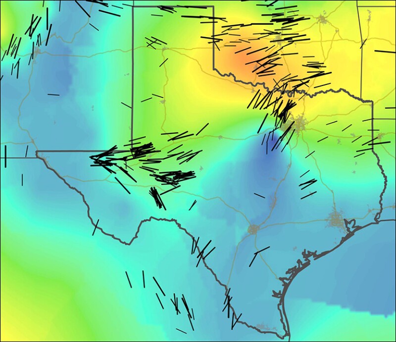
Elliott showed a map indicating what those regional stresses are like in Texas, New Mexico, and Oklahoma. The map, the product of a team of researchers at Stanford University led by seismology professor Mark Zoback, shows the differences between the maximum and minimum horizontal stresses.
Where that difference is greatest, such as it is in the Meramec play near Oklahoma City, is where Devon has found higher fracture-growth rates. Where the differences are smaller and faulting regimes are closer to normal, such as where Devon operates in the New Mexico portion of the Permian Basin, fracture growth is comparatively slower.
Elliott supposed that where stress anisotropy is highest, there “are less natural fractures that are capable of being opened,” which will impact how much fluid and pressure is able to leak off into the rock matrix.
The reverse is true where anisotropy is lower. In these geologies, more natural fractures are likely present and able to absorb more stimulation fluids closer to the wellbore. “We don’t have this solved,” said Elliott, “but it’s a very interesting and thought-provoking topic that has huge implications.”
A Fracture’s “Span of Influence”
Devon is working on ways to expand the value of SWPM and one of them involves tying the sealed wellbore data to fiber-optic strain data. The point is to see how much fracture area, along with the strain field generated inside the rock around a fracture, is physically impacting the monitor well. Devon calls this the “span of influence.”
This represents a notable new input for Devon since what it wants to do is to use as few stages as possible (i.e., as little capital as possible) to effectively stimulate a given portion of the reservoir.
Elliott showed a test between a single fracture cluster stage vs. one with five clusters. “Right off the bat, my eyes are drawn to the magnitude of responses,” he said of the multicluster stage design which resulted in “a much larger span of influence” over the monitor well.
This larger area of fracture activity also results in more casing deformation, which is critical to a related diagnostic approach Elliott is researching.
But with regard to the “span of influence” of fractures, Elliott said it boils down to “the sum of the strain, total/cumulative to that stage, and then we have [pressure from the] sealed wellbore monitors and we see a very nice, linear relationship there.”
Knowing this, Devon can push cluster and stage spacing further out, test it with fiber strain and SWPM, and determine the limits.
In one test the operator wanted to see what would happen when it used 150 ft-wide stages vs. 300 ft-wide stages. It found that for each respective length there was a nearly equal length of increased strain picked up by the fiber. If the stage was 150 ft in length, then the fracture appeared to be about 150 ft wide as it met the offset monitor. This was also true for the two 300-ft stages tested in the same well.
With this result, Elliott said, “We’ve proven to ourselves that we can extend that span of influence.”
Further, he pointed out that the data from SWPM and the fiber strain were in very strong agreement. As Elliott put it, “The biggest spans tied with the biggest response; the biggest-sum strain ties with the biggest sealed wellbore response.”
This learning might mean it is possible to use SWPM without the aid of fiber strain data to estimate how much fracture area touched a monitor well. Elliott is working on this as part of his PhD at the University of Texas at Austin.
The project, some details of which were published this year in SPE 209120, is trying to simulate the “subtle inflections and deformations” happening to the steel casing of the monitor well.
In severe cases the casing can be permanently deformed, which in and of itself is important to solve for. But what Elliot et al. are looking at is the much-smaller and less-damaging squeezes that wellbores feel anytime a fracture intersection takes place.
“When we’re talking about sealed wellbores, these pressure changes are being induced by millimeter changes, some are submillimeter,” Elliott explained. Understanding how those changes relate to the magnitude of oncoming fractures, and by simulating that, Devon can further scale SWPM to tune its injection volumes and rates to get a desired response.
Back to Injectivity Rates
Another relationship Devon is exploring is that between injection rates and the number of fractures created per stage. This goes back to the topic of cluster efficiency that SM Energy also raised at the conference.
Elliott pointed to a plot from one well showing pump rates between 5 and 30 bbl/min. In the latter case, fracture interactions happened significantly sooner than in the former.
Comparing this data with its fracture simulators has helped Devon validate the idea that a slower fracture arrival, or a delayed VFR, is a sign that fracture fluid is more evenly flowing through the various clusters.
“That’s kind of what we want to see,” added Elliott, who said Devon is developing yet another way to validate this by establishing a statistical relationship with all the possible fracture geometries a given VFR could generate between two wells.
In a field case, this approach was used to conclude that a VFR of 700 bbl that occurred in just 15 minutes likely resulted from one or two dominate fractures taking over in a stage with 14 clusters. This compared with a 20-cluster stage which saw almost 45 minutes pass before a VFR of more than 2,300 bbl was recorded on an offset monitor.
Elliott said not all 20 clusters achieved fracture growth, but likely 6 or 7 did and that allowed a threefold increase in stimulation fluid to enter the reservoir compared to the low-VFR case.
Based on the distributions of the probable solutions, he added that “it’s very unlikely that we have 12, 13, or 14 clusters generating that geometry, but it’s also unlikely that we have it all in one big, fat fracture.”
For Further Reading
SPE 209140 Multi-Pronged Diagnostics with Modeling to Improve Development Decisions—An Operator Case Study by Erich Kerr, SM Energy Company; Kyle Haustveit, Devon Energy; Reid Scofield, Erick Estrada, Andrew Johnson, and Scott Galuska, SM Energy Company; Jackson Haffener, Devon Energy; and Miles Landry, SM Energy Company.
SPE 209120 Integration of Sealed Wellbore Pressure Monitoring Responses with Wellbore Strain and Deformation Measurements for Fracture Diagnostics by Brendan Elliott, Devon Energy/UT Austin; Shuang Zheng, Rod Russel, and Mukul Sharma, UT Austin; and Kyle Haustveit and Jackson Haffner, Devon Energy.
SPE 204140 An Eagle Ford Case Study: Monitoring Fracturing Propagation Through Sealed Wellbore Pressure Monitoring by Kourtney Brinkley, Trevor Ingle, Jackson Haffener, Philip Chapman, Scott Baker, Eric Hart, Kyle Haustveit, and Jon Roberts, Devon Energy.