
In Australia’s Surat Basin, gas is contained in hundreds of coal seams, which have highly variable properties and are grouped into four distinct reservoir zones of similar qualities. Economically producing these wells from multiple reservoir units is generally favored and as a result, understanding the relative contribution to production by different zones at different times in the well’s life—and whether production is dominated by a single zone—adds value to planning future wells.
The well designs are quite simple. An 8.5-in. wellbore is drilled from surface casing through the target coal seams. A 7-in. production casing and preperforated liner with an external casing packer and a cement stage tool is run to total depth. The external casing packer is deployed at the top of the reservoir, and the 7-in. casing is cemented in place through the stage tool above the packer. No external packers are installed between groups of coal seams (zones) to segregate production from each zone through the preperforated liner.
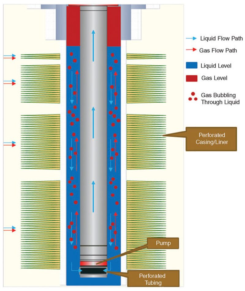
Production tubing is installed in the well, which typically runs to the base of the preperforated liner, and a progressive cavity pump (PCP) is installed in the tubing to lift the water produced with the coal-seam gas (CSG) [dewater the well]. Gas production comes from the coal seams and flows around and through the preperforated liner, then up through the annular space, between the production liner/casing and the production tubing, to surface. The water flows to the bottom of the completion, where it is lifted up the production tubing by the PCP as shown in Fig. 1 above.
Understanding Zonal Allocation
Normally, production logging tools (PLTs) are run to obtain an understanding of zonal allocation in commingled wells. However, running PLTs in CSG wells can be expensive as it requires the PCP to be pulled out and the well to be lifted with gas. The switch to gas lift at shallow depth is not a normal operating condition and may affect the result.
An additional issue is the unsegregated, openhole completion. With no external packers, neither the PLT tools nor the distributed-temperature sensor (DTS) fibers inside the liner can measure flow in the space between the liner and the sandface.
A DTS application from a fiber-optic cable is a potential solution to the challenges of using PLTs. For DTS use, a light pulse is transmitted down the fiber-optic cable in the well. The light is reflected by imperfections in the fiber, and a permanent interrogator on the surface can calculate the relative temperature from intervals as small as 0.5 m to 1 m going down the fiber.
The data set of temperature with depth is then collected over time. In addition to fiber installations run on the outside of the tubing, fiber can also be installed on the outside of the preperforated liner, as close to the formation as possible.
To analyze the reservoir flow using DTS technology, an operator installed fiber in multiple wells and connected them to a permanent interrogation unit on the surface. Typically, temperature profiles were recorded every 6 hours and transmitted to a cloud-based database for immediate visualization and analysis.
The commercially available software FloQuest was used as it allowed for visualization of a large amount of DTS data in combination with gauge and log data for easy comparison, event mining, and identification. The built-in modeling tool also meant that both visualization and modeling could be done within the same package.
Many of these wells have now had more than a year of DTS data collected, which covers shut-in, preproduction, the initial dewatering with single-phase water, and initial gas production and ramp-up periods.
Temperature Model
Changes in the temperature profiles of production wells are usually dominated by two major factors: the effects of flow commingling and heat transfer. Assuming no chemical interaction between the fluids, the final temperature after commingling is calculated by following the principles of energy conservation. However, evaluating the heat loss to the formation is more complex, as there is the possibility of annular bidirectional flow with water flowing down while gas bubbles upward through it to the surface.
To reduce the complexity, modeling was carried out only on traces logged during the dewatering period that had single-phase flow (SPE 171545). Inflow temperature is taken to be the same as that of the geothermal and as such, it is important to obtain a good initial geothermal temperature profile.
The set of inflow rates that delivers a match to observed temperature profiles describes the inflow profile of the well. The calculated rates are then used to achieve the corresponding permeabilities of the zones. To assess the validity of a DTS interpretation, the results can be compared with permeability measurements made from sensors in nearby wells. An example of this is shown for a single point in time in Fig. 2, which shows the DTS-logged temperature in a well with single-phase water production.
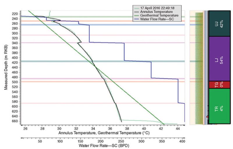
The gas rate was also verified from gauge data. As shown in Fig. 2, a very good match between modeled and observed temperature can be achieved. As is the case for any history-matching activity, a non-unique solution is delivered that is subject to some uncertainty. For instance, a different geothermal gradient assumption would necessitate different inflow rates to achieve a match.
Measured data (light-green curve), has been matched by the modeled temperature (black curve) by varying the water produced from different horizons. It can be seen that the modeled wellbore temperature matches the measured temperature closely. The four producing formations are: upper Juandah (UJ), lower Juandah (LJ), Tangalooma (TG), and Taroom (TR).
DTS data for two additional dates from the same well were matched with FloQuest models. This DTS result was then compared with the reservoir-modeled behavior for the well. In this case, the reservoir model populated by static drillstem testing measurements behaved in a similar way to the dynamic DTS data.
The flow rate contributions interpreted from the DTS system were found to be approximately 40–60% (UJ, LJ), 0–15% (TG), and 0–5% (TR). The flow rate contributions seen from analysis of the reservoir model, averaged over the producing period, were 58% (UJ), 38% (LJ), 2% (TG), and 1% (TR). This example for one well shows the insight possible with DTS measurements.
Liquid Level in the Well
Before production, the well had a full water column to ground level. As the pump removed water from the well, the column fell and drawdown on the formation was initiated. The DTS system recorded temperature data above and below this liquid level. The liquid depth level during normal operations is generally kept as deep as possible by pumping off the water to create the largest drawdowns on the formation. This means it is common for the reservoir section to be partially covered by a water column and have gas to surface in the casing (liner)/tubing annulus.
This complicates the temperature data from DTS measurements. The most confident DTS interpretations are from periods when the liquid column was kept above the reservoir section, although this is not representative of standard well operations.
Depletion Trends
Because DTS systems record temperature throughout the life of the well, events that may not be investigated by a PLT campaign can be observed. All wells showed crossflow events when shut in, and with confidence established in the geothermal gradient, the direction of crossflow can be inferred. Assessing trends across areas can provide an indication of which horizons deplete the fastest. Post-production shut-ins from two wells were compared, with both showing the same behavior of shallower coals flowing to deeper intervals. It can be postulated that the deeper coal intervals have been depleted more by production than the upper coals.
Conclusion
Accurate zonal allocation from DTS data has been demonstrated during single-phase water production periods. DTS temperature data can be collected continuously during well life, allowing the tracking of the phasing of production from different horizons and the analysis of shut-in behavior. This can provide an understanding of crossflow behavior and subsequent interpretation of the zonal contribution and depletion.
Challenges have been encountered when trying to quantify zonal allocation. Having only one data set (temperature with depth), the flow behind a preperforated liner, an uncertain geothermal gradient, and having a fluid level below the top perforation all add complexity to DTS interpretation.
With multiphase gas and water production, temperature modeling becomes more complicated and quantitative zonal allocation that is based on DTS temperature data alone is not currently possible. There is potential that as wells move to single-phase gas conditions, a new thermal model can provide zonal allocation data.
It is also recognized that supplementary data from fiber could improve the understanding of zonal allocation. Combining the interpretation of DTS data with that of distributed acoustic sensing data may provide a solution to the flow allocation challenge.
Reference
SPE 171545-MS The Application of Advanced Wellbore Monitoring in Coal Seam Gas for Continuous Inflow Profiling by G. Naldrett et al.
The article is an abridged copy of paper SPE 186203-MS, which was presented at the SPE/IATMI Asia Pacific Oil & Gas Conference and Exhibition held in Bali, Indonesia, 17–19 October 2017.