
The coupling of hydraulic fractures and natural-fracture networks and their interaction with the shale matrix remains a major challenge in reservoir simulation and modeling of shale formations. This article reviews methods used to understand the complexities associated with production from shale to shed light on the belief that there is much to be learned about this complex resource and that the best days of understanding and modeling how oil and gas are produced from shale are still ahead.
Introduction
Preshale Technology. The phrase “preshale” technology aims to emphasize the combination of technologies that are used to address the reservoir and production modeling of shale assets. In essence, almost all of the technologies used today for modeling and analysis of hydrocarbon production from shale were developed to address issues that originally had nothing to do with shale. As the shale boom began, these technologies were revisited and modified in order to find application in shale.
Conventional Discrete Fracture Network. The most common technique for modeling a discrete natural fracture (DNF) network is to generate it stochastically. The common practice in carbonate and some clastic rocks is to use borehole-image logs to characterize the DNF at the wellbore level. These estimates of DNF characteristics are then used for the stochastic generation of the DNF throughout the reservoir.
The idea of the DNF is not new. It has been around for decades. Carbonate rocks and some clastic rocks are known to have networks of natural fractures. Developing algorithms and techniques to generate DNFs stochastically and then couple them with reservoir-simulation models was common practice before the so-called “shale revolution.”
A New Hypothesis on Natural Fractures in Shale
What are the general shapes and structures of natural fractures in shale? Are they close to those of the stochastically generated set of natural fractures with random shapes that has been used for carbonate (and sometimes clastic) formations? Or are they more like a well-structured and well-behaved network of fractures that have a laminar, plate-like form, examples of which can be seen in outcrops (such as those shown in Fig. 1)?
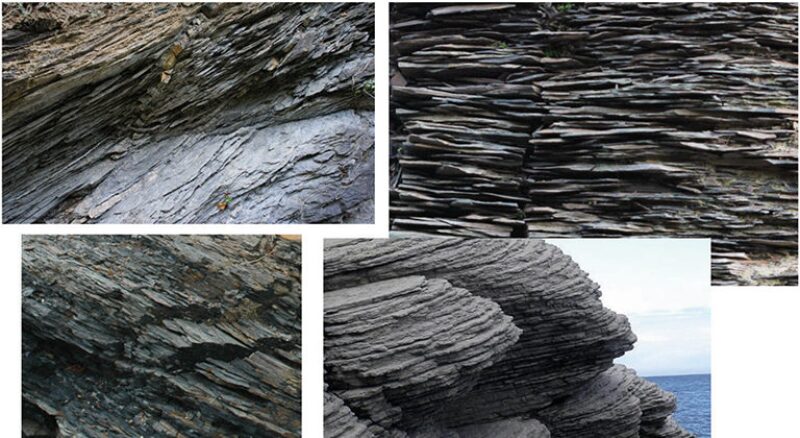
Shale is defined as a fine-grained sedimentary rock that forms from the compaction of silt and clay-sized mineral particles commonly called mud. This composition places shale in a category of sedimentary rocks known as mudstones. Shale is distinguished from other mudstones because it is fissile and laminated.
If such definitions of the nature of shale are accepted and if the character of the network of natural fractures in shale is as observed in the outcrops, then many questions must be asked, some of which are
- How would such characteristics of the network of natural fractures affect the propagation of the induced hydraulic fractures in shale?
- How would the production characteristics of shale wells be affected by this potentially new and different way of propagation of the induced hydraulic fractures (compared with how we model them today)?
- What are the consequences of these characteristics of natural fractures on short- and long-term production from shale?
- How would this affect current models?
- What can it tell us about new models that need to be developed
Reservoir Simulation and Modeling of Shale
The current state of reservoir-modeling technology for shale uses the lessons learned from modeling naturally fractured carbonate reservoirs and those from coalbed-methane reservoirs. The combination of flow through double-porosity naturally fractured carbonate formations and the concentration-gradient-driven diffusion that is governed by Fick’s law integrated with Langmuir isotherms that control desorption of methane into the natural fractures has become the cornerstone of reservoir modeling in shale.
The presence of massive, multicluster, multistage hydraulic fractures only makes the reservoir modeling of shale formations more complicated and makes the use of current numerical models even less beneficial. Because hydraulic fractures are the main reason for economic production from shale, modeling their behavior and their interaction with the rock matrix becomes one of the more important aspects of modeling storage and flow in shale formations.
All the existing approaches of handling massive, multicluster, multistage hydraulic fractures in reservoir modeling can be divided into two distinct groups: the explicit hydraulic-fracture (EHF) -modeling method and stimulated reservoir volume (SRV).
EHF Modeling
EHF modeling is the most complex and tedious (as well as the most robust) approach for modeling the effect of hydraulic fracturing during numerical simulation of production from shale. The modeling technique couples three different technologies and consists of the following steps:
- Modeling the effect of the hydraulic fracture
- Developing a geological model
- Incorporating fracture characteristics in the geological model
- Completing the base model
- History matching the base model
- Forecasting production
SRV Modeling
SRV modeling is a different and much simpler way of handling the effect of massive, multicluster, multistage hydraulic fractures in numerical reservoir simulation and modeling. Using SRV modeling instead of EHF modeling can expedite the modeling process by orders of magnitude. This is because, instead of meticulously modeling every individual hydraulic fracture, the modeler assumes a 3D volume around the wellbore with enhanced permeability as the result of the hydraulic fractures. By modifying the permeability and dimensions of the SRV, the modeler can now match the production behavior of a given well in a much shorter time.
The sensitivity of production from shale wells to the size and the conductivity assigned to the SRV explains the uncertainties associated with forecasts made with this technique. Although attempts have been made to address the dynamic nature of the SRV by incorporating stress-dependent permeability, the entire concept remains in the realm of creative adaptation of existing tools and techniques to solve a new problem.
Making the Case for Full-Field Reservoir Simulation and Modeling of Shale Assets
A quick look at the history of reservoir simulation and modeling reveals that developing full-field models (where all the wells in the asset are modeled together as one comprehensive entity) is common practice for almost all prolific assets.
Looking at the numerical reservoir-simulation modeling efforts for shale assets, one cannot help but notice that almost all of the published studies are concentrated on analyzing production from single wells.
The argument to justify the limited approach (single well) to modeling of shale assets concentrates on two issues: the computational expense and the lack of interaction between wells because of the low permeability of shale. The argument about the computational expense is quite justified. Those who have been involved with numerical modeling of hydrocarbon production from shale can testify that modeling even a single well, which on the average includes 45 clusters of hydraulic fractures (15 stages assuming three clusters per stage), can be an extreme challenge to set up and run. If EHF modeling is used, the model can take tens of hours for a single run; therefore, building a geological model that would include details of every cluster of hydraulic fractures for an asset with hundreds of laterals is computationally prohibitive.
While the first reason (computation expense) seems to be legitimate and realistic, the second reason is merely an excuse with limited merit. It is well-established that shale wells do communicate with one another during production. It has been shown that communication occurs between laterals from the same pad as well as the laterals from offset pads. The “frac hit” is a common occurrence of such interaction. A “frac hit” is when injected hydraulic-fracturing fluid from one well shows up at another well and interferes with its production.
Data-Driven Modeling of Production From Shale—An Alternative Solution
Because analytical and numerical full-field modeling of shale assets is either impractical or leaves much to be desired, data-driven modeling provides an alternative solution. Top-down modeling (TDM) is the application of predictive data-driven analytics to reservoir modeling and reservoir management.
TDM has been defined as a formalized, comprehensive, multivariant, and full-field empirical reservoir-simulation and modeling approach that is specifically geared toward reservoir management. In TDM, measured field data (and not interpreted data)—hard data—are used as the sole source of information to build a full-field model, treating and history matching each well individually. This approach minimizes interpretation of the data and relies heavily on all that is known and measured in the field.
TDM uses the production history of each individual well in the asset along with wellhead pressure. The production data are augmented by all the hard data that are collected during drilling, logging, and completion of each well. All the parameters that are measured during the hydraulic fracturing are incorporated into the top-down model, such as type and amount of fluids that are injected, type and amount of proppants, and injection pressures and corresponding injection rates. The top-down model is history matched for every well in the asset. Once training, calibration, and validation of a top-down model are complete, its use is similar to that of conventional full-field models.
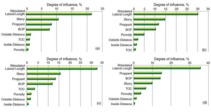
The final top-down model has a small enough computational footprint to allow for a comprehensive sensitivity analysis. Results of some of the sensitivity analyses performed on a specific pad are shown in Fig. 2. The advantages of using data-driven technology to perform reservoir modeling are
- No assumptions are made regarding the physics of the storage and production of hydrocarbon in shale
- Hard data is used to perform modeling instead of soft, interpreted data
- Use of hard data instead of soft data makes it possible to use this model to design optimum fracturing jobs
- The small computational footprint allows for full-field analysis as well as sensitivity and uncertainty analyses
- More wells and more data make model development more reliable and more robust
The disadvantages of using data-driven technology include
- Not being able to explain explicitly the storage and transport phenomena in shale
- Data-driven modeling is not applicable to an asset with few wells (approximately 10 to 20 wells are required to start data-driven modeling)
- Long-term prediction of the production from a given well is not a simple and straightforward process.
This article, written by Special Publications Editor Adam Wilson, contains highlights of paper SPE 165713, “A Critical View of Current State of Reservoir Modeling of Shale Assets,” by Shahab D. Mohaghegh, SPE, Intelligent Solutions and West Virginia University, prepared for the 2013 SPE Eastern Regional Meeting, Pittsburgh, Pennsylvania, USA, 20–22 August. The paper has not been peer reviewed.