

A year ago, I wrote a JPT Guest Editorial on stripper wells in the US. It was the result of data analysis that I personally found shocking and the result of frustration I was having with clients looking for acquisitions at that time.
The piece was written right before oil prices started an incredible climb and when natural gas prices had been under $3.00/Mcf for an extended period. On the acquisition and divestiture front, although corporate consolidation was ongoing, deal counts were at a decade low, and it was extremely hard to transact. With oil prices at $45/bbl and the so-called “shale bust” of the past few years, many investors would not even consider an unconventional asset.
Given this backdrop, I had clients on the hunt for conventional assets with stable base cash flow and limited risk. One client was a very serious buyer; however, some decision makers were adamant about certain asset characteristics, namely conventional, onshore US, certain states, operated working interest, proved producing (PDP), and no stripper wells. Despite this seeming like a reasonable set of criteria, asset after asset kept getting screened out. Finally, I had a call with the CFO and in frustration told him, “They’re all stripper wells.”
Something about saying that out loud stuck in my head and got me thinking. I started wondering “how many stripper wells are there?” I began to think about the well count across the US, well IPs (initial production or starting flow rates), and the approximate rates at which I generally saw most wells go uneconomic in financial modeling. Given about 1 million active wells in the US, it seemed like there ought to be a decent percentage of active, producing, conventional wells over the 20–30 BOPD mark. I started pulling well data and found that for many US regions, 95% or more of the active vertical wells were producing 15 BOPD or less.
The article generated a lot of interest as it brought to light something many people think is a problem in the back of their mind but had not seen quantified in a simple way. The follow-up question I got over and over was “What about horizontal wells?”
The US Energy Information Administration (EIA) estimates that about 80% of US oil and gas wells are producing less than 15 BOEPD. For horizontal wells, EIA estimates about half are 50 BOEPD or less (the use of 6:1 BOE tends to improve the overall daily rate in an amount that is disproportionate to the value and economic impact of adding the gas stream). This rate includes both conventional and unconventional wells. It is natural to assume that the older conventional wells bring down the average and that more recent production from the hottest US shale plays is much higher.
In the following analysis I look specifically at unconventional horizontal wells. These are wells that are drilled vertically down to a kickoff depth and then drilled outward along a targeted geological feature. The wells are drilled down to varying depths and then outward for significant distances—often 1 to 2 miles. Unconventional wells are hydraulically fractured due to the type of rock in the targeted formations, resulting in fractures that are held open by proppant and serve as conduits for flow in rock that would otherwise be too tight for oil and gas to move through.
The principles behind unconventional wells lead to very different production profiles from conventional wells. When you drill a big horizontal well and fracture it, there is a rush of oil out of the fractures. This gives you very high IPs. However, this rush of production is just that—a rush. Large volumes come out at first but subside in a relatively short amount of time. The initial unloading of the fractures only lasts a few years in most cases and is followed by much lower rates of production for the remaining life of the well.
I think about it as a freeway in Houston for the fractures and a Colorado dirt road for the so-called matrix. Once the fractures have unloaded, there is still production but it is much less and much slower. These are big, expensive wells that cost more than vertical wells to operate and if they are dropping to much lower rates in a matter of a few years, it begs the questions : How many in the US are currently considered low rate? And under what conditions are they economic to produce?
Fig. 1 shows the oil production profile for a sample set of unconventional wells in Midland County, Texas. For this set of wells production has already dropped to one-tenth of the IP in only 3 years.
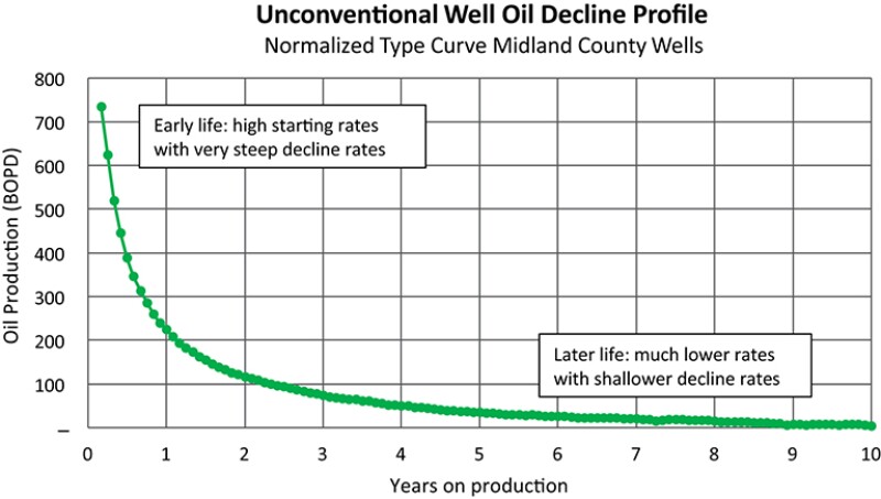
Fig. 1 uses a normalized curve which is similar to averaging. Wells are all lined up at their first-month production, the rates at month 1 are added up, and then the total rate is divided by the well count that month. It represents the “average” production of a well in its first month and subsequent months to give an overall idea of behavior across the group. Normalized curves are then fit with a smooth line through the data to give type curves. The outcome is highly dependent on the sample set or group of wells and there are many important considerations in choosing groups. These results give a high-level overview. In-depth analysis requires additional considerations such as well counts, lateral lengths, benches, and typically, reservoir engineer forecasting.
Fig. 1 includes wells from the past 13 years; however, improving well technology and completions optimization over the years has tended to result in higher IPs. Fig. 2 shows the wells grouped by year.
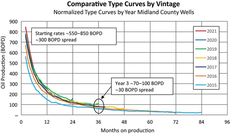
As shown in Fig. 2, despite improvements in IP these wells collapse in both rate and spread in as few as 3 years. Well economics and investments look much different at 700 BOPD than they do at 70 BOPD. With such a dramatic change in a relatively short time, there is increasing industry concern about what to do with later-life unconventional wells.
Unconventional Well Production Distribution in Key US Plays
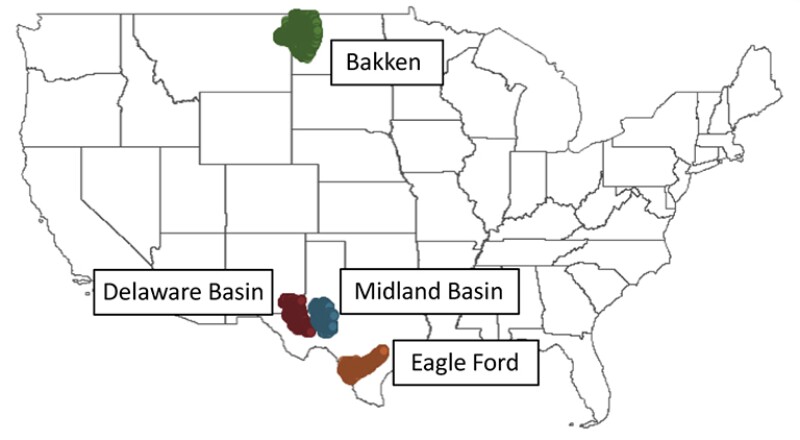
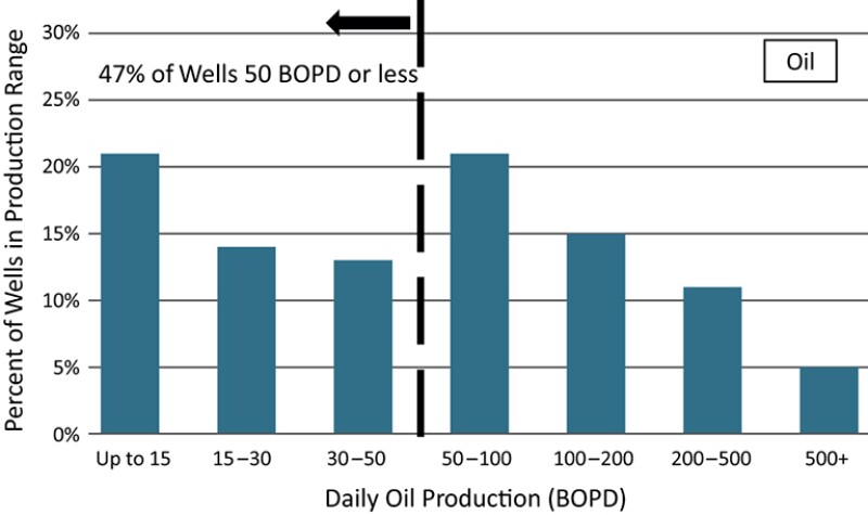
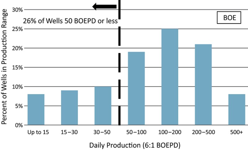
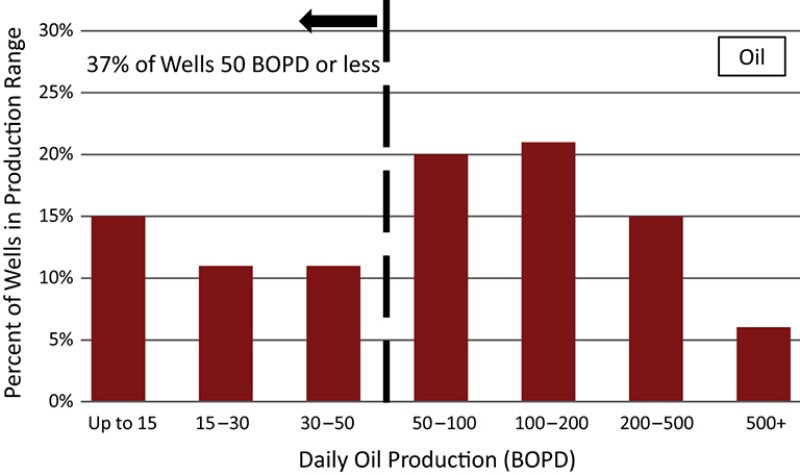
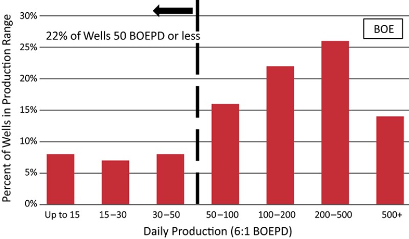
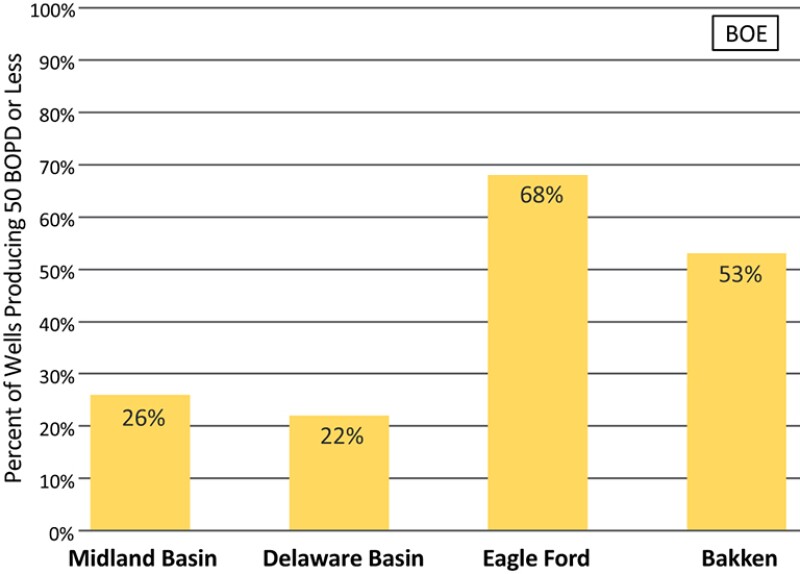
This analysis looks at four major US unconventional plays. The Permian is split into the Midland Basin and Delaware Basin; the Eagle Ford; and the Bakken. Oil and 6:1 BOE are shown separately. The 6:1 BOE conversion represents energy equivalency in Btus; however, this ratio is not reflective of well economics—specifically, the number of Mcfs of gas you would have to sell to make the same amount of money as selling 1 bbl of oil. At today’s spot prices of $93.10/bbl and $3.94/Mcf you would have to sell approximately 24 Mcf of gas to get the same amount of money as 1 barrel of oil. The use of 6:1 BOE tends to make the rates look higher, but the rate increase is disproportionate to the value and economic impact of adding the gas stream. Study wells are shown in Fig. 3.
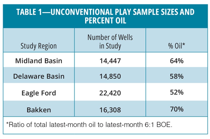
The results are based on average daily production for the latest month. The last 12-month daily production was reviewed and did not significantly change the results. The 50 BOPD and 50 BOEPD dividers are not representative of economic limit calculations. As shown in Figs. 1 and 2, by the time many wells are down at 50 BOPD or lower, they are well past their prime. The 50 BOEPD limit demonstrates the impact of adding gas product streams at 6:1 BOE. Natural gas liquids are excluded due to the limited availability of public data. Sample sizes and percent oil are shown in Table 1.
Note for Figs. 4–13. Enverus DrillingInfo (DI) data with DI classifications: plays as shown in Fig. 3, horizontal wells, classified as active, 0s excluded (under 0.01 BOEPD), binned by average BOPD and BOEPD for latest month production, greater than lower bound and up and including higher bound, sample sizes in Table 1, public allocated data typically an individual well basis—may include separately reported completions or lease-level data divided by well count, limited to unconventional reservoirs. Permian plays include DI classification for reservoirs that include Trend Area, Wolfcamp, Spraberry, or Bone Spring. Bakken and Eagle Ford are limited to DI reservoirs containing Bakken or Eagle Ford, respectively.
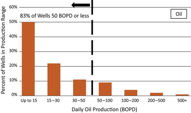
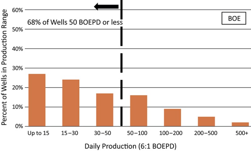
MIDLAND BASIN (14,447 TOTAL WELLS)
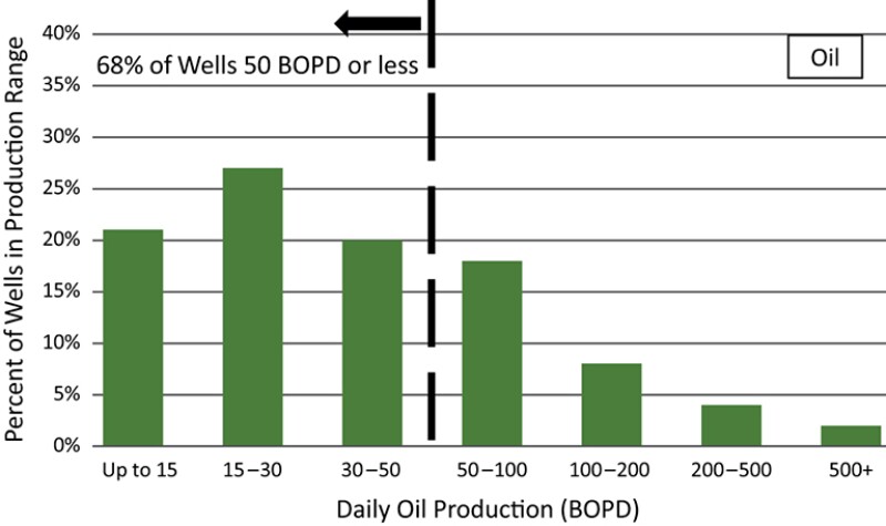
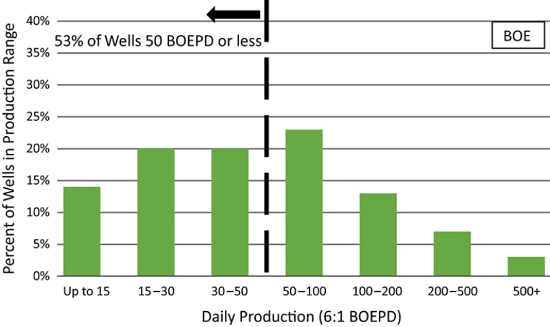
DELAWARE BASIN (14,850 TOTAL WELLS)
EAGLE FORD (22,420 TOTAL WELLS)
BAKKEN (16,308 TOTAL WELLS)
MAJOR US PLAYS (68,025 TOTAL WELLS)
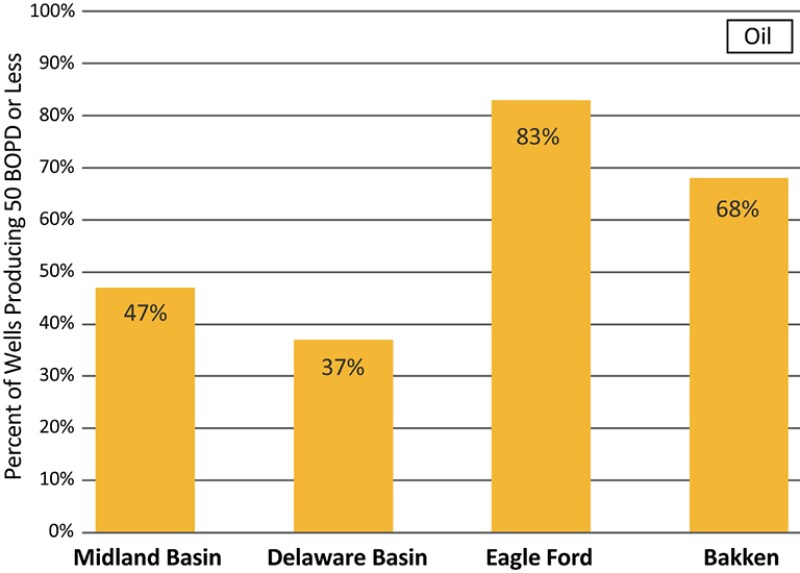
The results show a significant percentage of unconventional wells aging out into lower production rates even in the most active and hottest US basins. As shown in Figs. 1 and 2, by the time most wells are down at 50 BOPD rates they are well past their prime. Economic viability of these wells varies based on many inputs including commodity prices, price differentials, fixed and variable operating expenses (opex), and overhead (G&A). At today’s oil prices many unconventional wells can be produced down into the 10–20 BOPD range and still show a positive PV10.
One of the key considerations for lower-rate unconventional well economic limits is the cost of a workover when the well goes down. The lower the production rate, the longer the payout period becomes. Given the cost and probability of success, there comes a point when the economics no longer work for big horizontal well workovers. Some companies are trying to turn the tide on later-life wells with refracs and enhanced oil recovery, but so far these have had mixed results.
In comparison to my article on vertical conventional wells, horizontal unconventional wells across key US plays appear to have significantly better longevity at this time. However, we are at high commodity prices. Also, ongoing opex and full plugging and abandonment with reclamation are typically much higher for unconventional wells than conventional wells. As greater numbers of unconventional wells age out there is increasing concern about how to operate them profitably and about the growing asset retirement obligations across the entire US oil and gas industry.
